Cs194-26 Project 1
Colorizing the Prokudin-Gorskii Collection
Norman Karr | nkarr11@berkeley.edu
Norman Karr | nkarr11@berkeley.edu
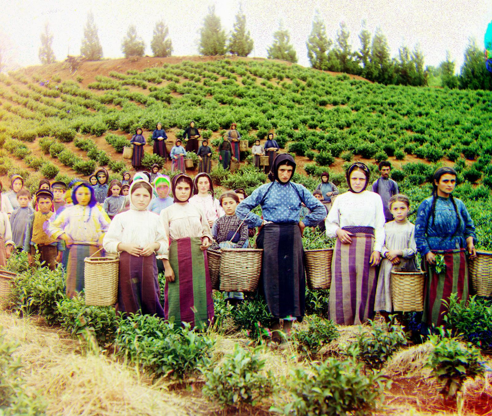
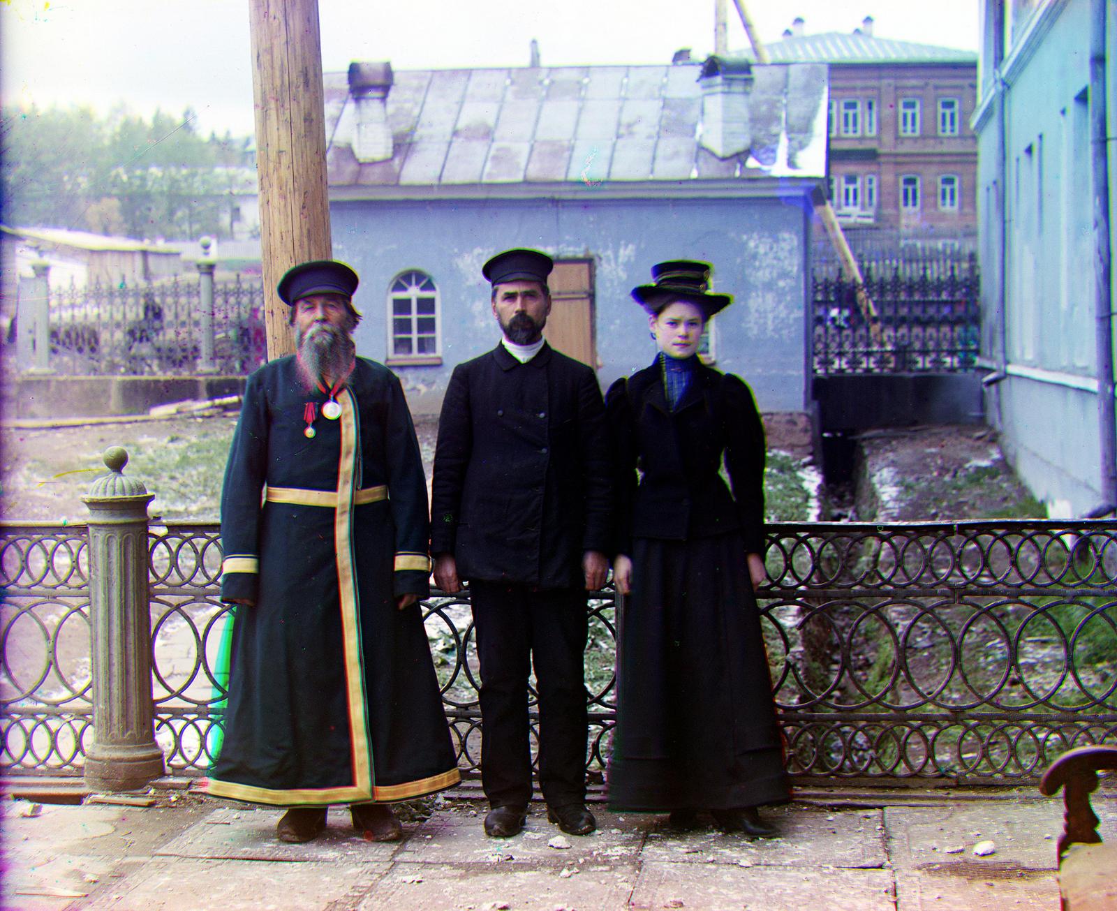
In 1907, a man by the name of Sergey Mikhailovich Prokudin-Gorskii took three exposures of every single scene he photographed. One exposure had a red filter, one had a green filter, and the last one had a blue filter. Together, three three images represent the activations of each color channel. The goal of this project was to create a automated pipeline that would combine the three exposures of each image to generate a vibrant, colorized image of each photograph.
1. Alignment Metrics
2. Pyramid Search
4. Edge Alignment
5. Further Endeavors
1. Smart Cropping
2. Sharpening
3. Contrast
4. Further Endeavors
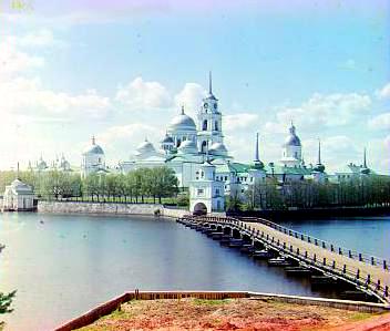
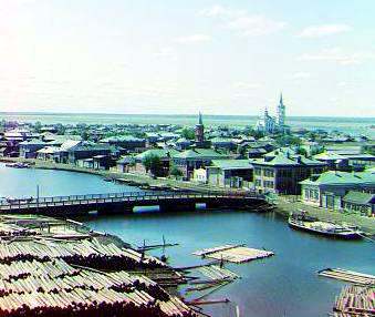
1. Final Images
2. Offset Values
3. Fun Results
Let's turn three grayscale images into one color image. That doesn't sound crazy at all!
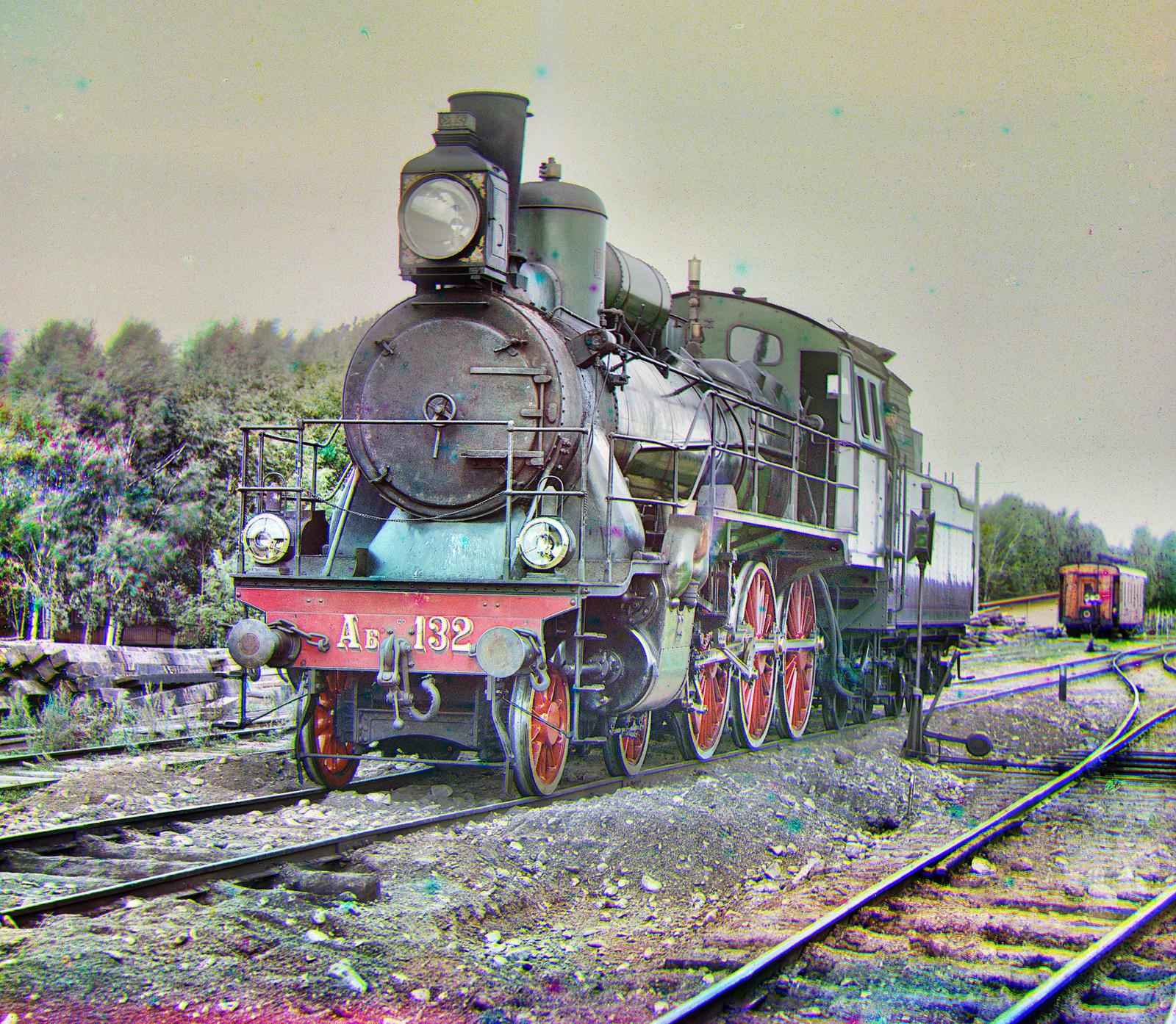
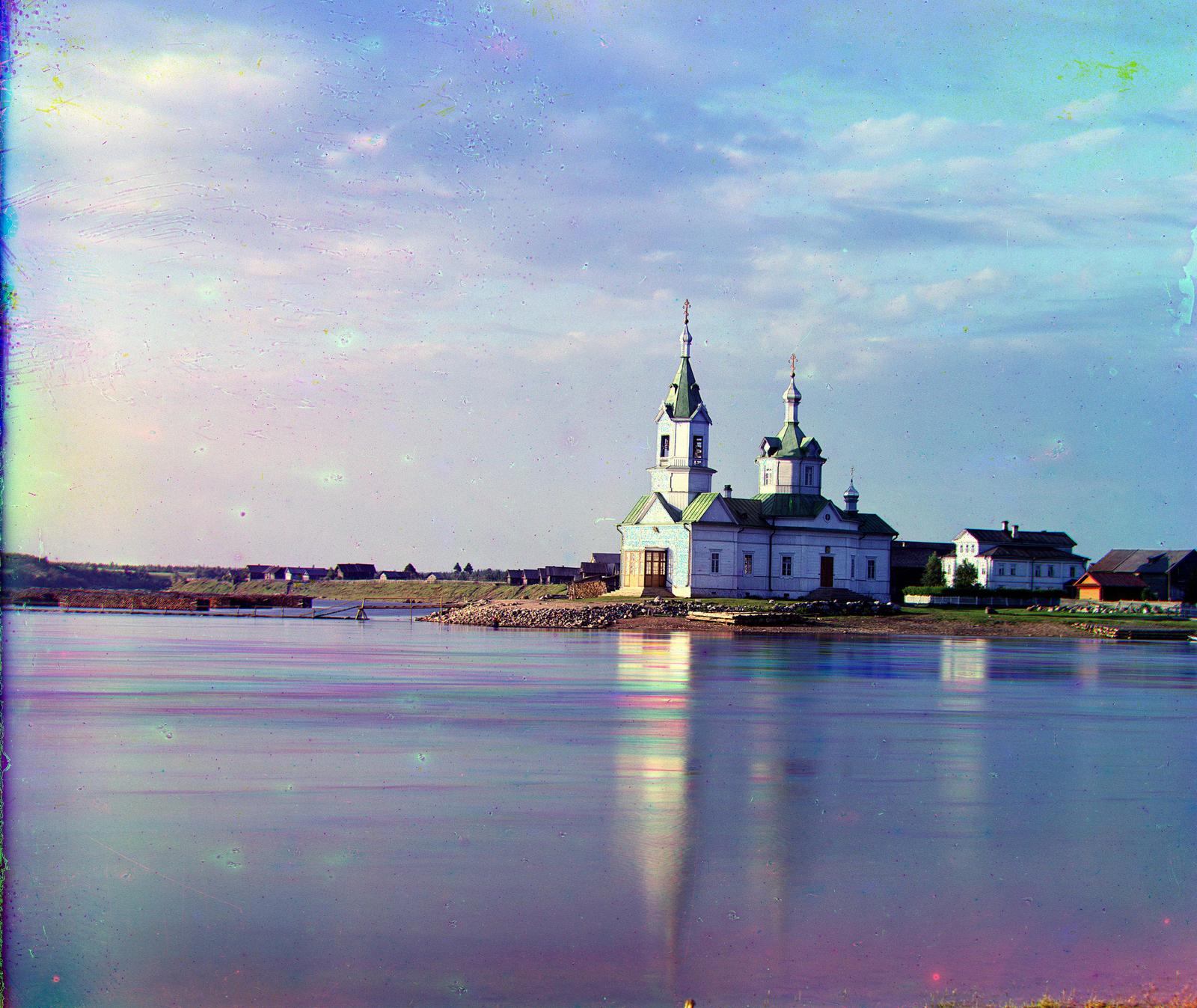
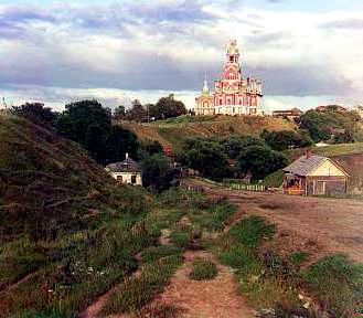
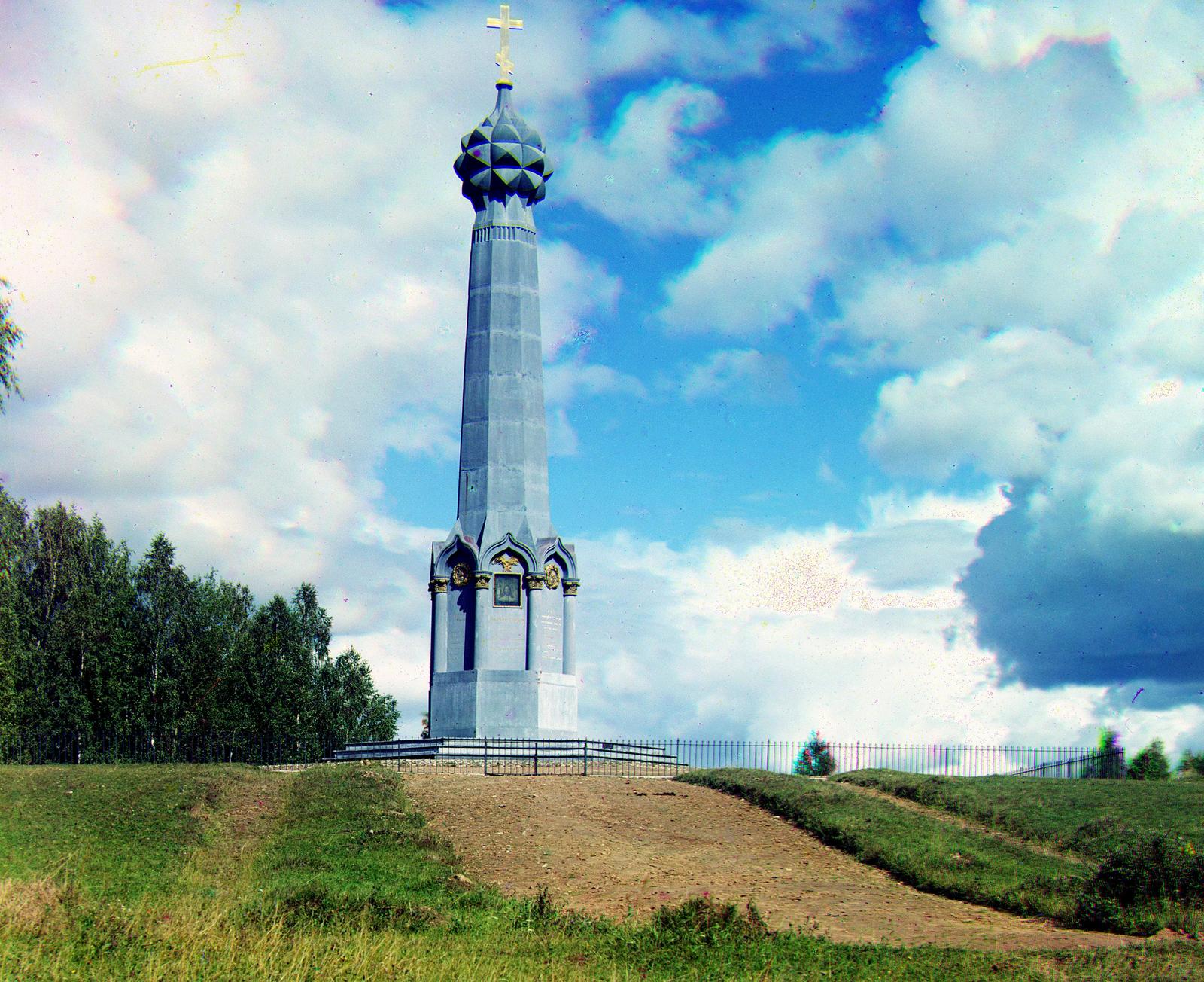
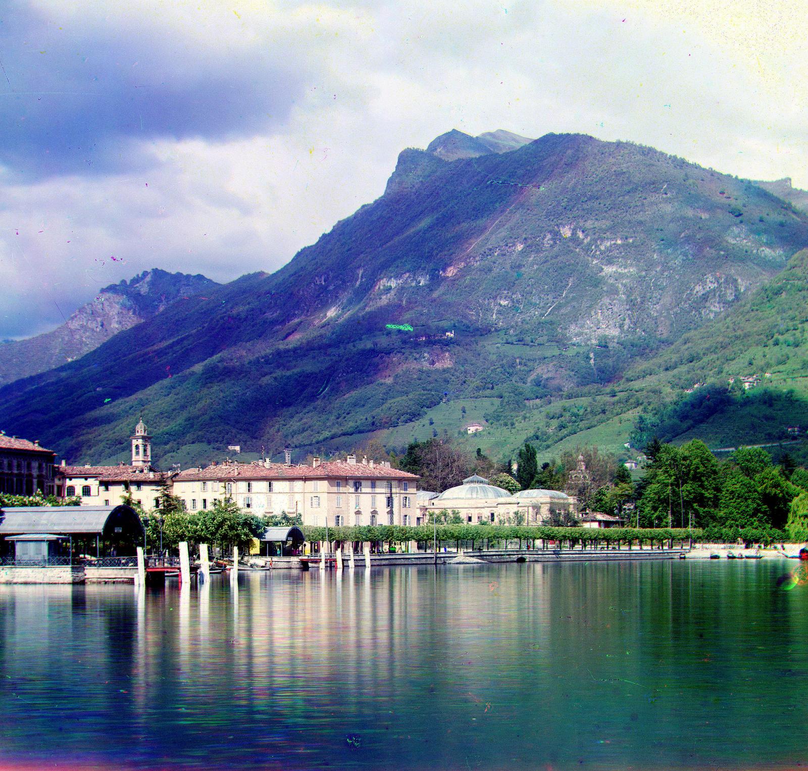
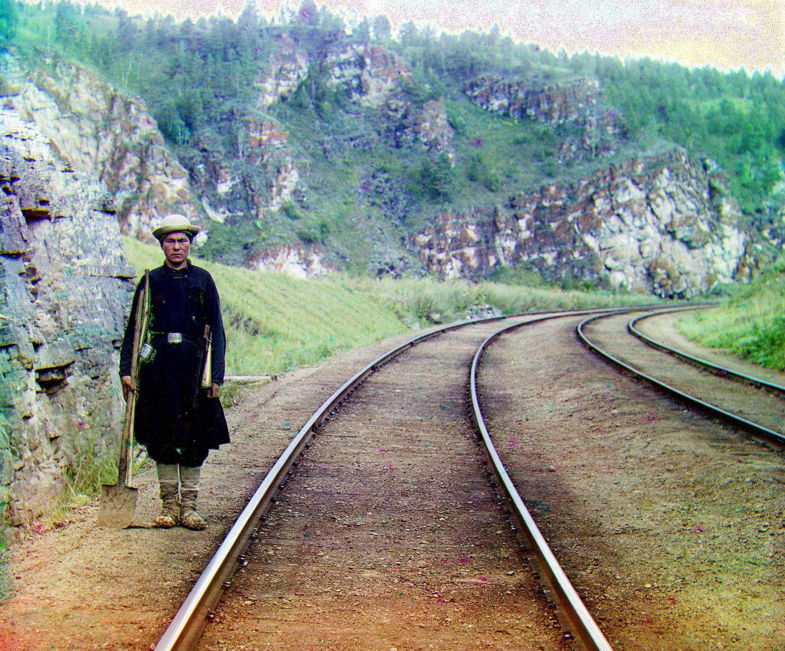
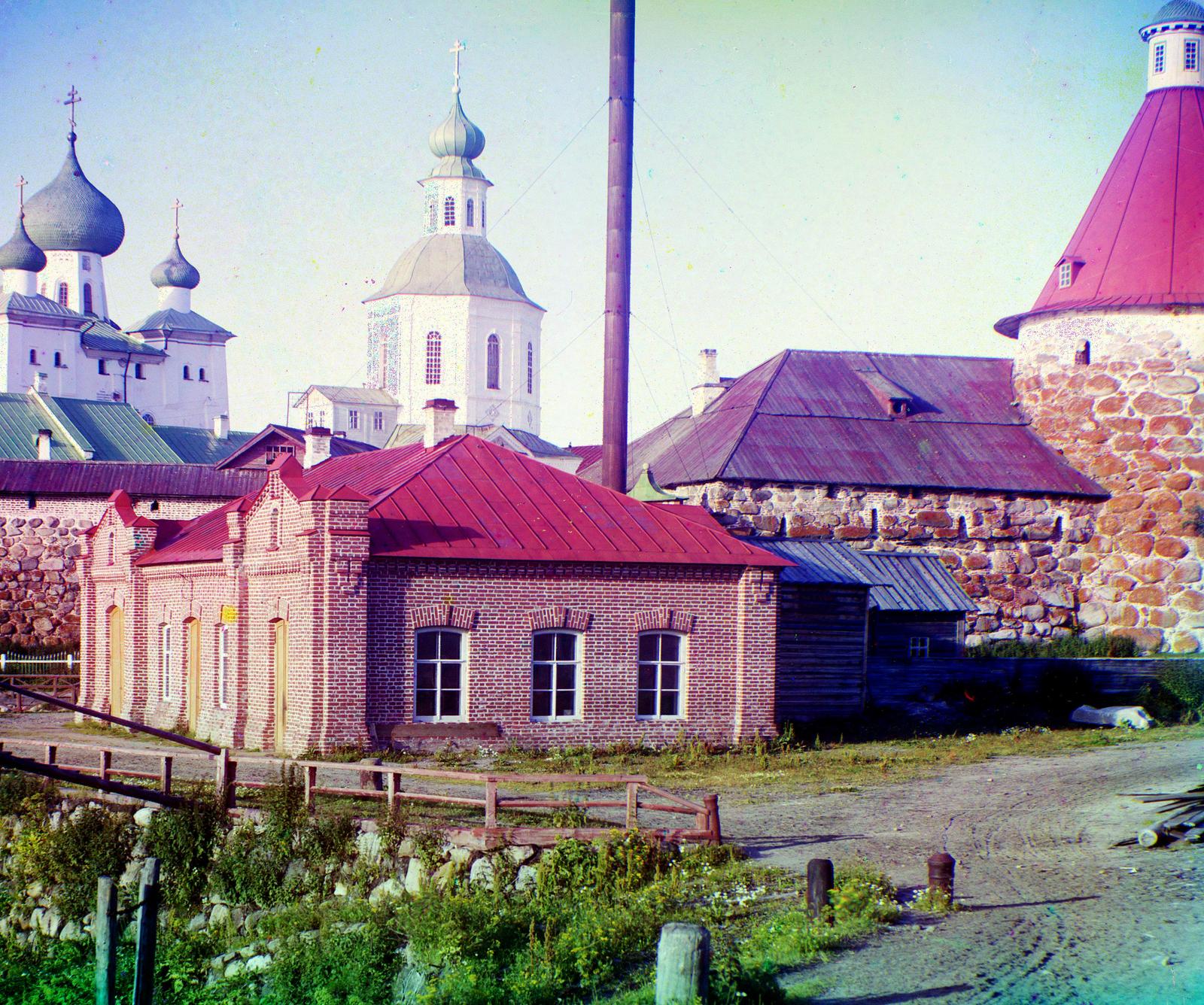
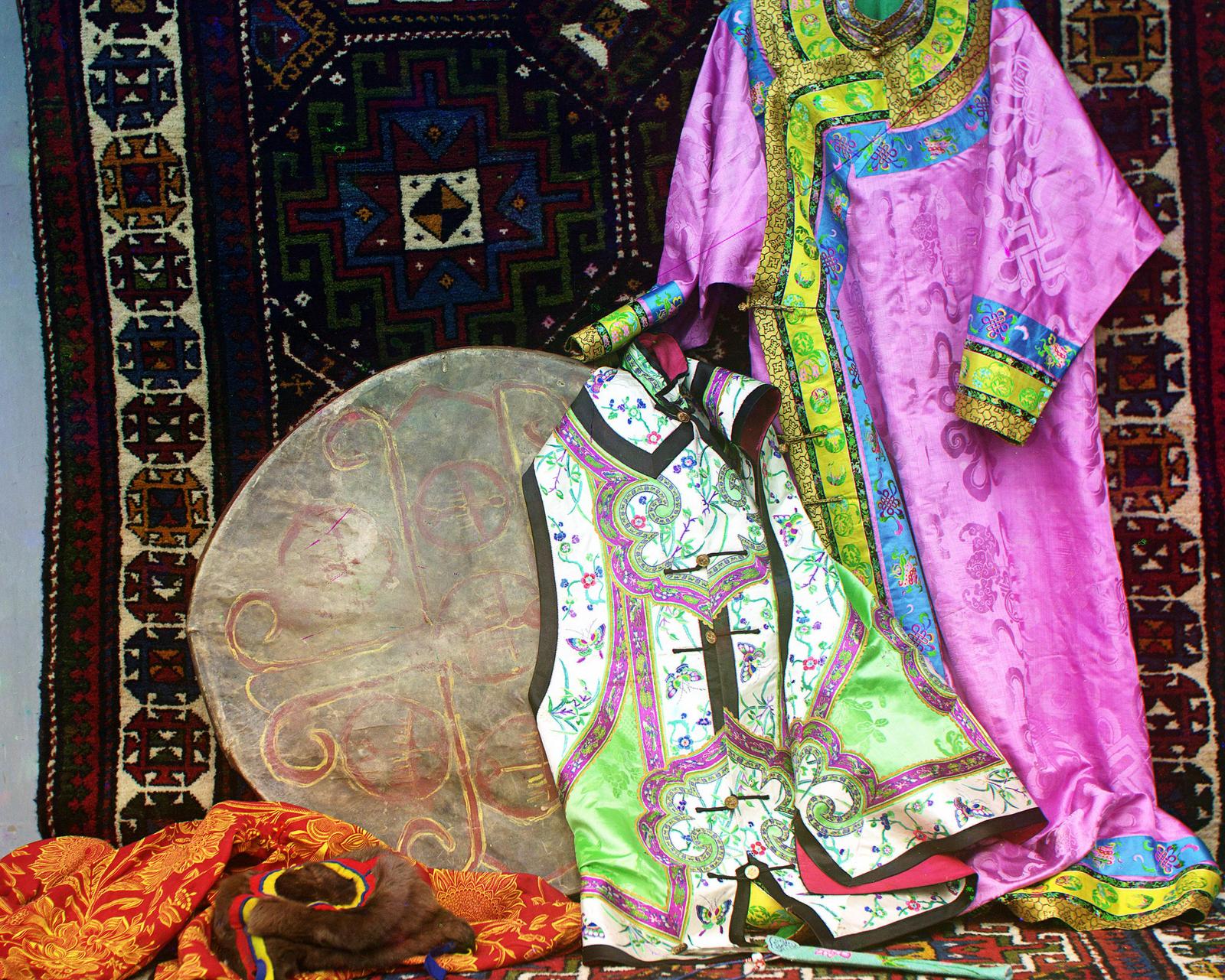
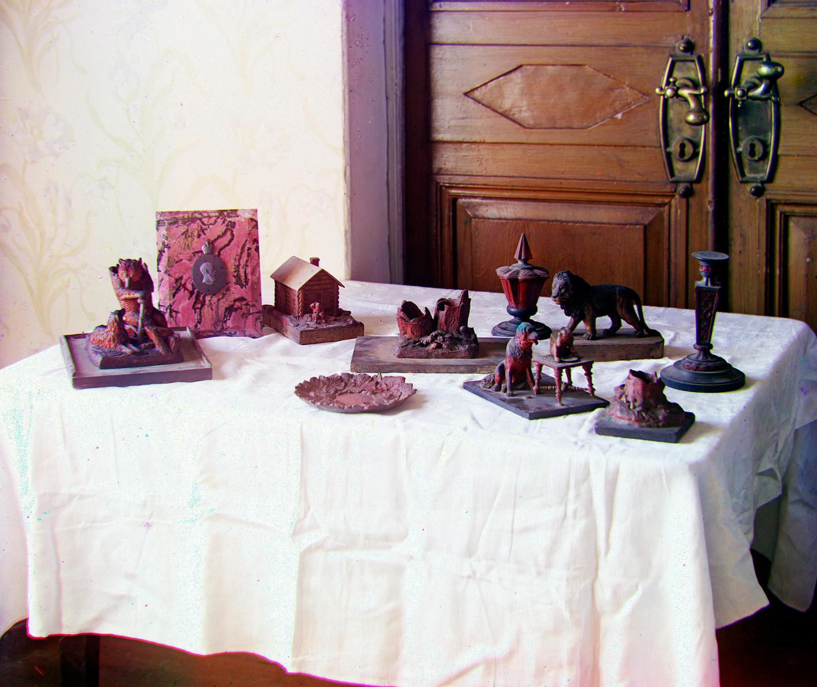
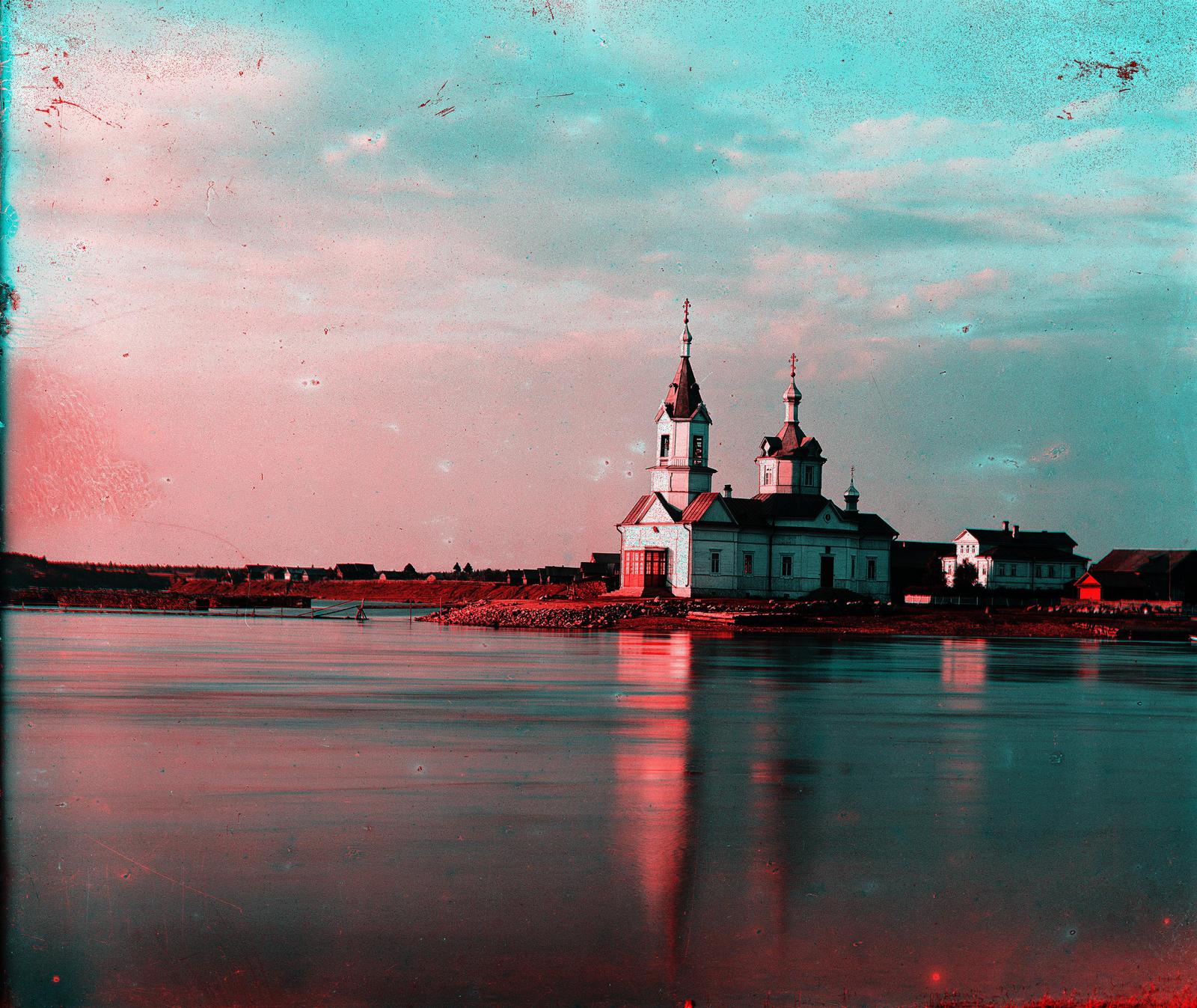
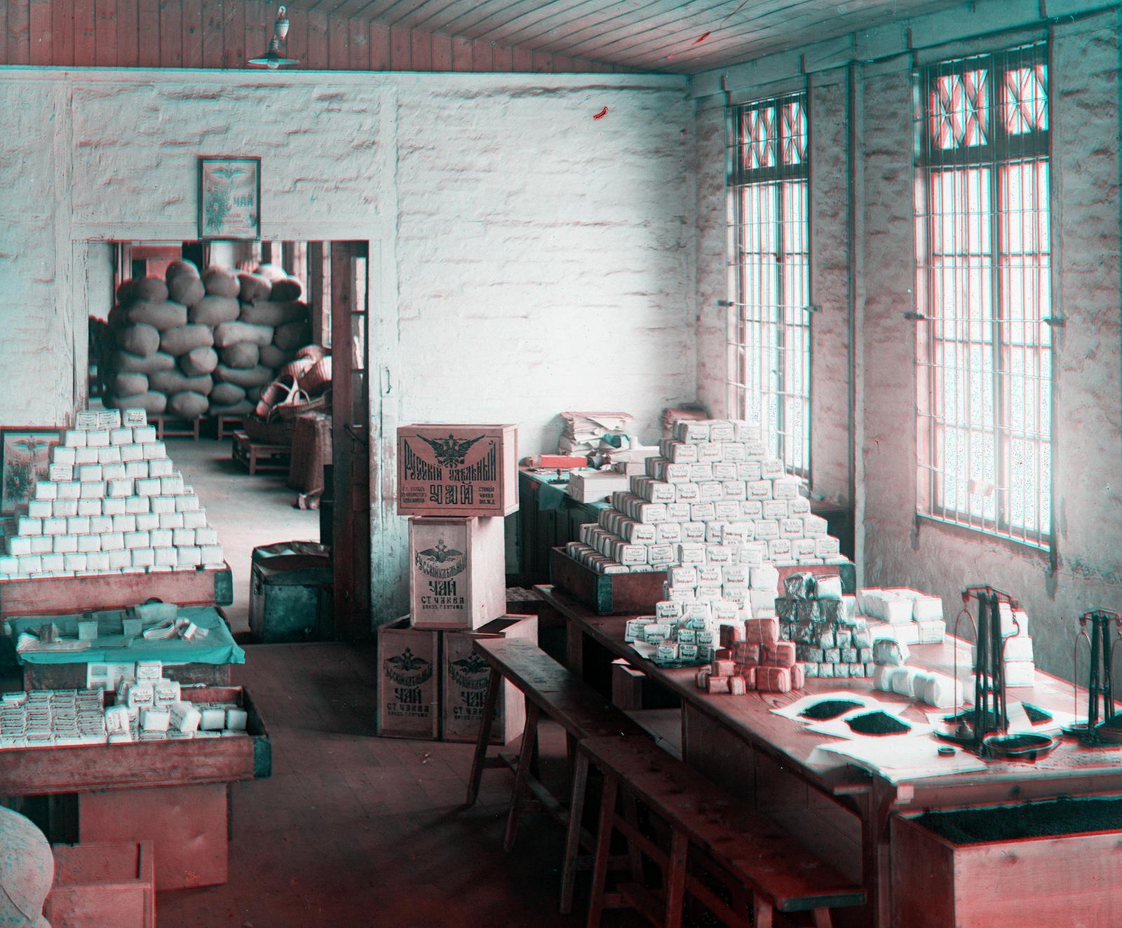
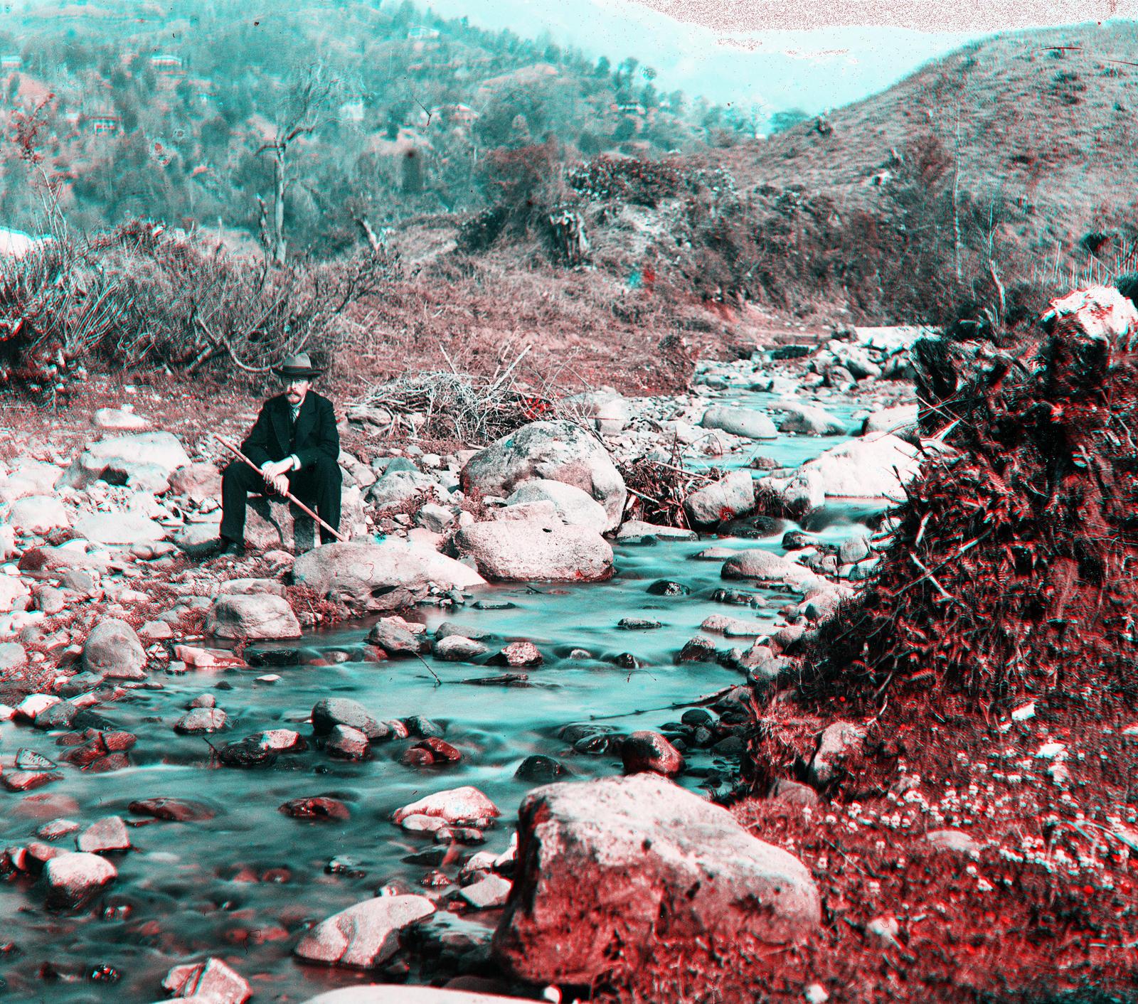
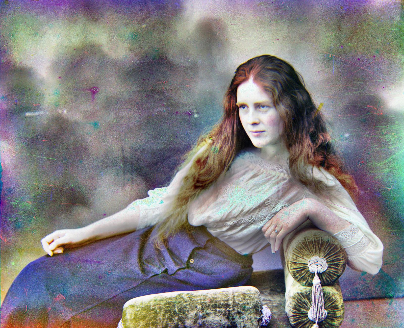
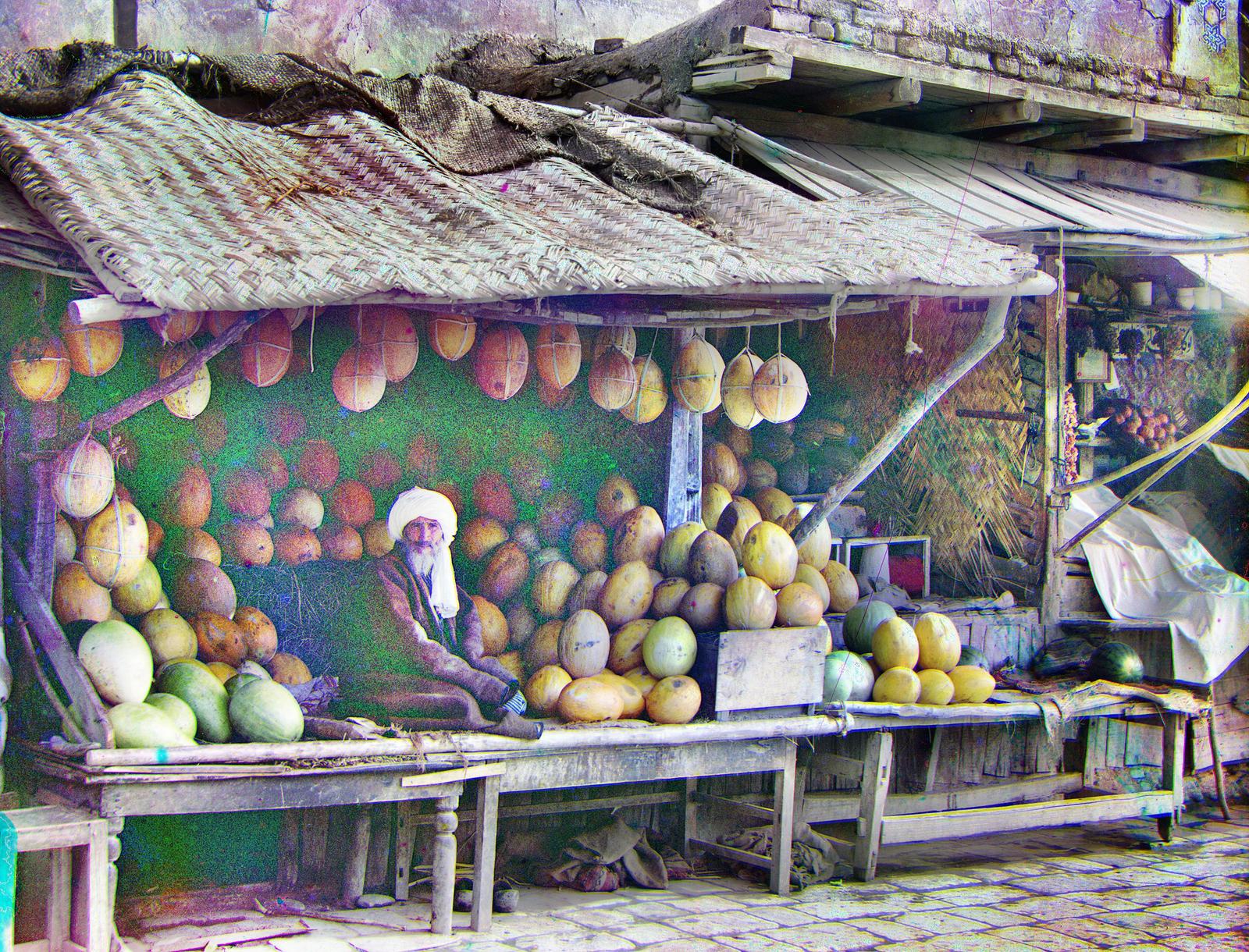
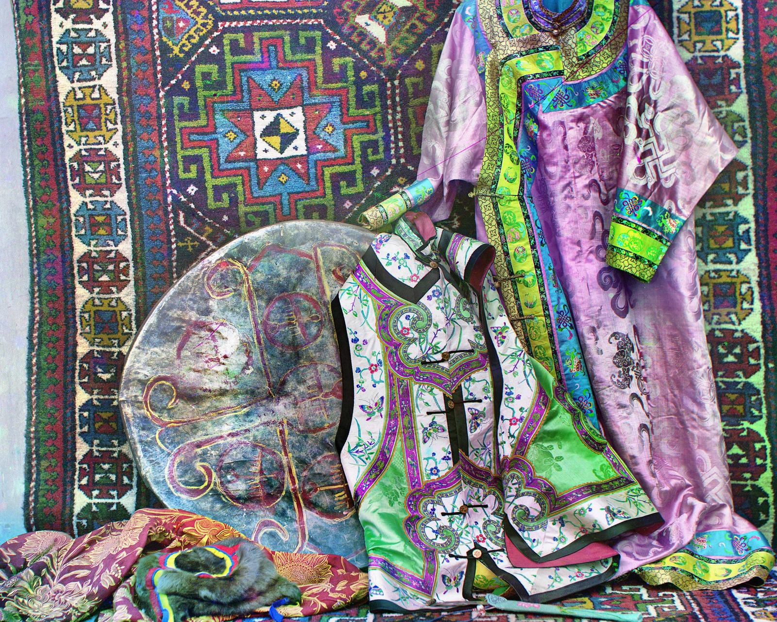
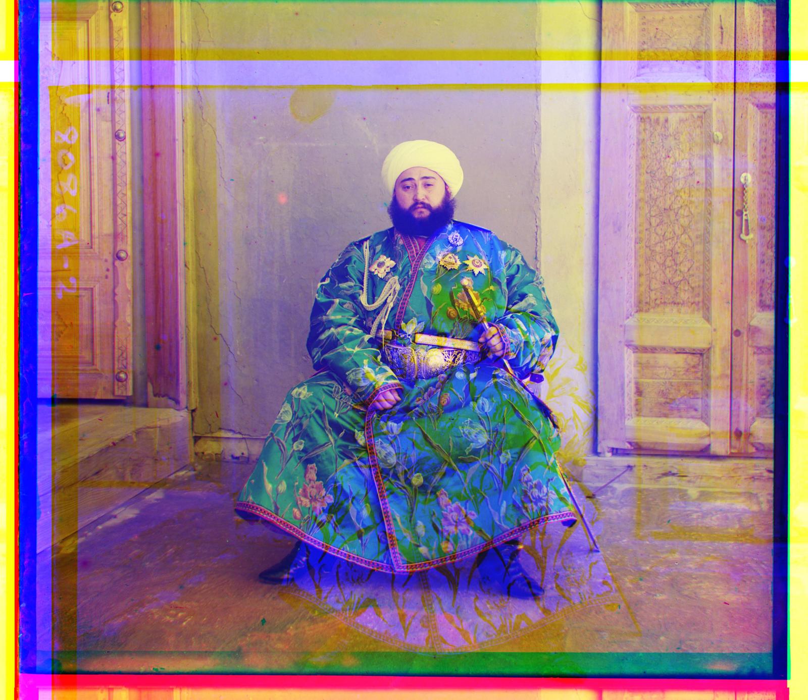
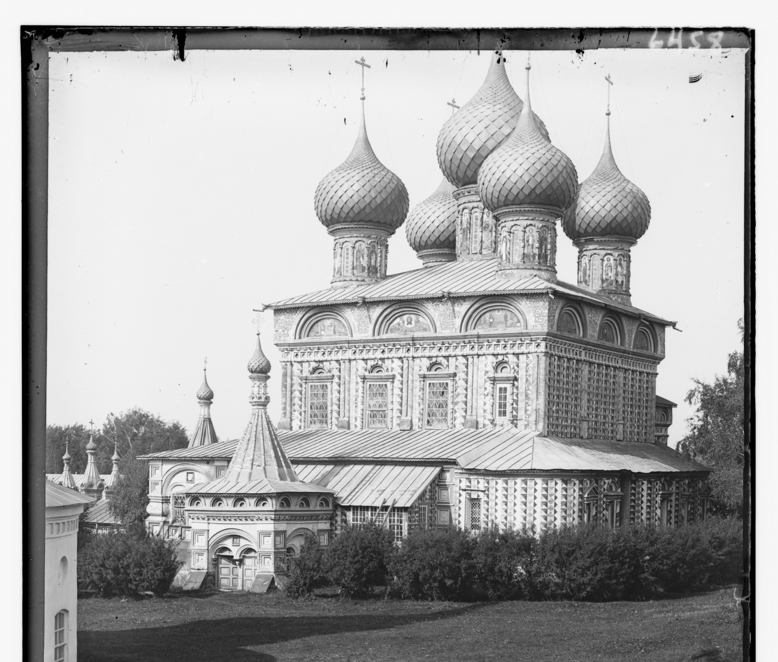
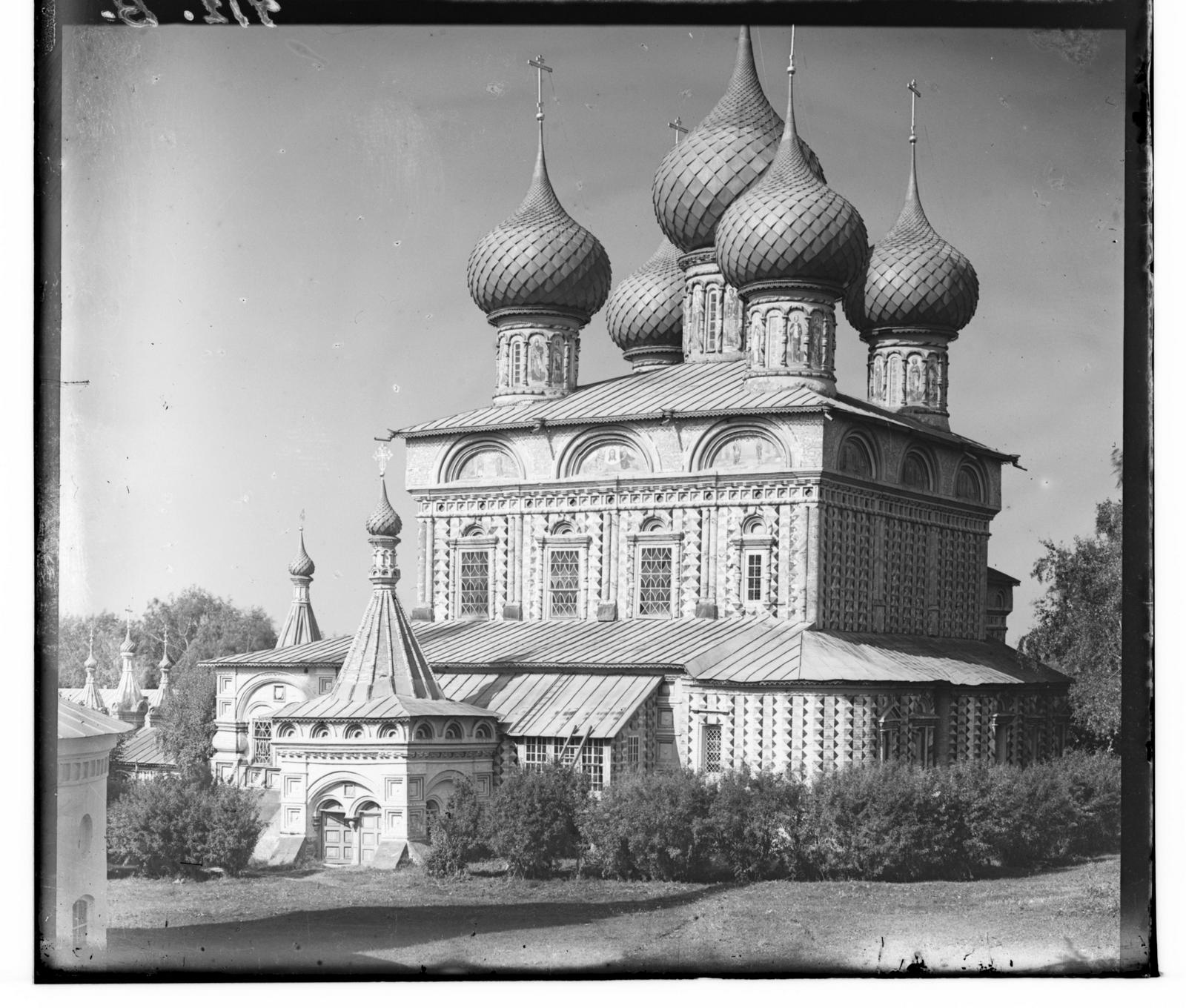
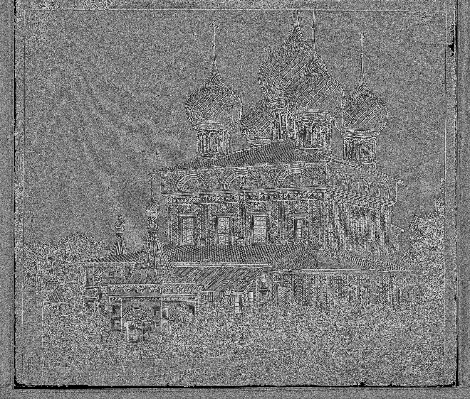
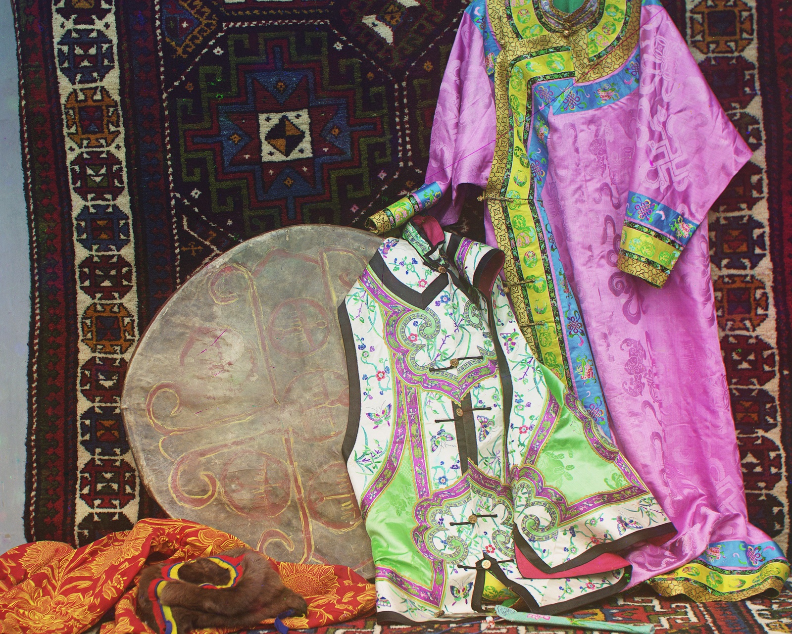
Before we go into the methodology, let's take a look at the data we are given:
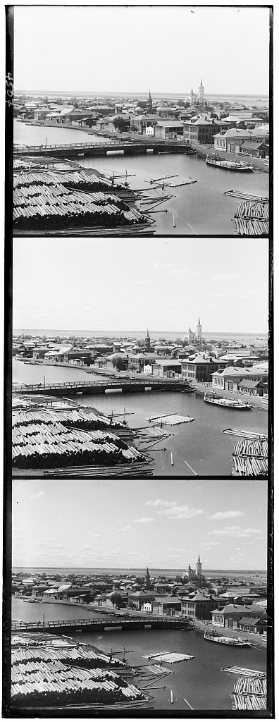
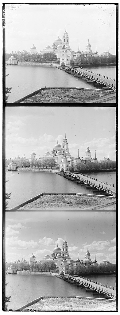
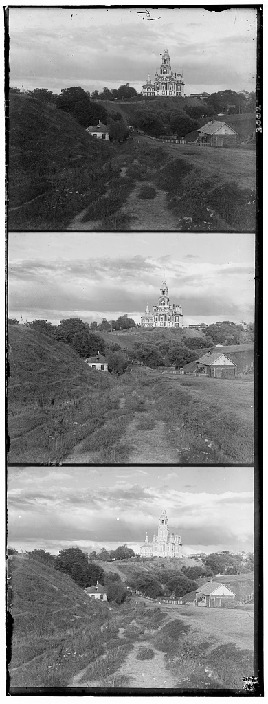
Our given data is awesome and it's really kind of crazy how different each photo is per filter. Our goal is to split these film exposures into their respective channels and then align them. One thing to note before moving on to alignment is that the order of filters in the images from top to bottom is actually blue, green, red (not the conventional red, green, blue).
The natural first step in figuring out how to align images is to come up with a numerical metric that can measure how well aligned two images are. Fortunately, there are two relatively simple solutions to this. The first metric is a pixelwise L2 norm, or sum of squared differences (SSD) which is calculated by taking the pixelwise difference between two images and returning the squared norm of the result. The second metric is a normalized cross-correlation (NCC) which is just a dot product between two normalized images.* In my experiments, I found that NCC produced better results than SSD the majority of the time but took twice as long to calculate.
*To increase consistency, I decided to use a negative NCC so that both of my metrics become minimization problems.
Unfortunately, both of these metrics are made to compare two objects, not three. As a result, we have to treat one color channel as a reference channel and then use the metrics to align the other two channels to our reference. For example, if the red channel is our reference, we will align the blue to the red and then align the green to the red. Interestingly, selecting different references actually results in different alignments. After some experiments, I found that using the green channel as the reference channel produced the most consistent results.
One shortcoming of blindly applying the metrics is the pixel instability in the borders of each image. Since the borders are so irregular, these areas of the image would contaminate the accuracy of the metrics. To avoid the borders, I employed a crop of each image before calculating the alignment accuracy. For each image, I evaluate the metrics only on the middle 60% of each image.
To test different alignments, I exhaustively iterate through a [-10,10] pixel offset range in both the x and y direction. This strategy is sufficient for small images but fails for larger images because the true offset can be greater than ±10 pixels. Unfortunately, this exhaustive search becomes way too slow when we increase the range to say [-100,100]. I solved this issue by employing an algorithm known as pyramid search.
One obvious issue with directly aligning pixel activations is that not all parts of an image will have the same activation in each channel. If this was the case, then our colored image would be actually black and white. To increase alignment robustness, I opted to perform alignments based on edges in the image instead. To do this, I convolved each channel with an edge detection kernel and then aligned each image based off of the edge detection activations.
One shortcoming is that the alignment is currently limited to a x and y offset. Possible explorations could include adding a search through different scales, rotations, and sheers to further improve alignment. To employ a search through more dimensions requires significant improvement to my algorithms' speed.
Another specific thing I would like to explore is a more intelligent search other than exhaustive searching. One idea I had was calculating some sort of gradient of SDD or NCC with respect to my parameters. This way I can more intelligentally approach optimal values with gradient descent as opposed to exhaustively searching through a space.
Now that our images are aligned and in color, how can we make the images better?
In each of our aligned photos, there is often a border that is pure black, pure white, or some other extreme color. I wanted to find an intelligent way to crop the images dynamically such that we only see the clean, center image. For this, I employed a custom algorithm to crop out these unwanted borders.
The next effect in my pipeline is a sharpening function which I perform by simply convolving every image with a sharpening kernel. This function only works for larger images and although minor, the difference is noticable when viewing the .tif files. After compressing to a jpeg, the difference is even less noticable however if you look very closely, you can still tell that some edges became more sharp. Regardless, automatic sharpness operates on each image that passes through my pipeline.

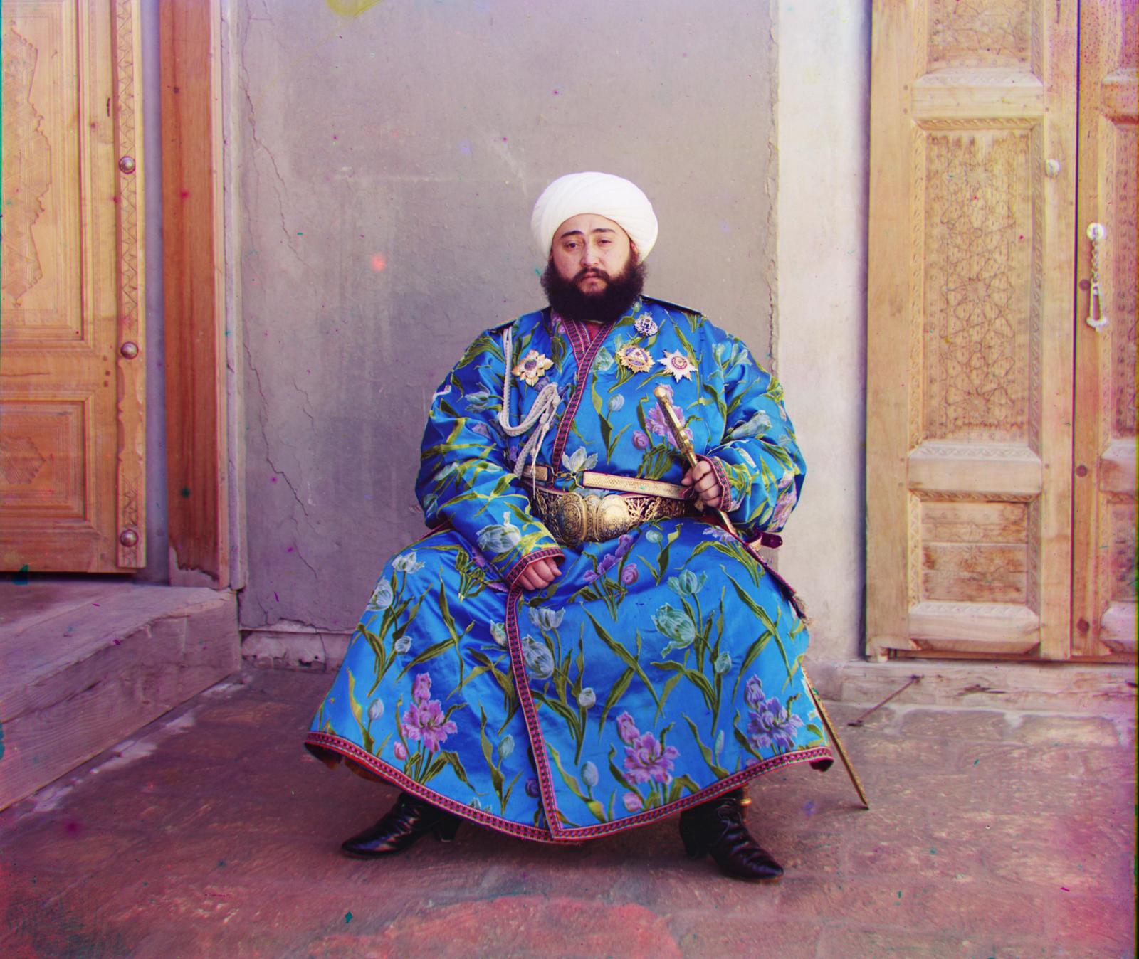
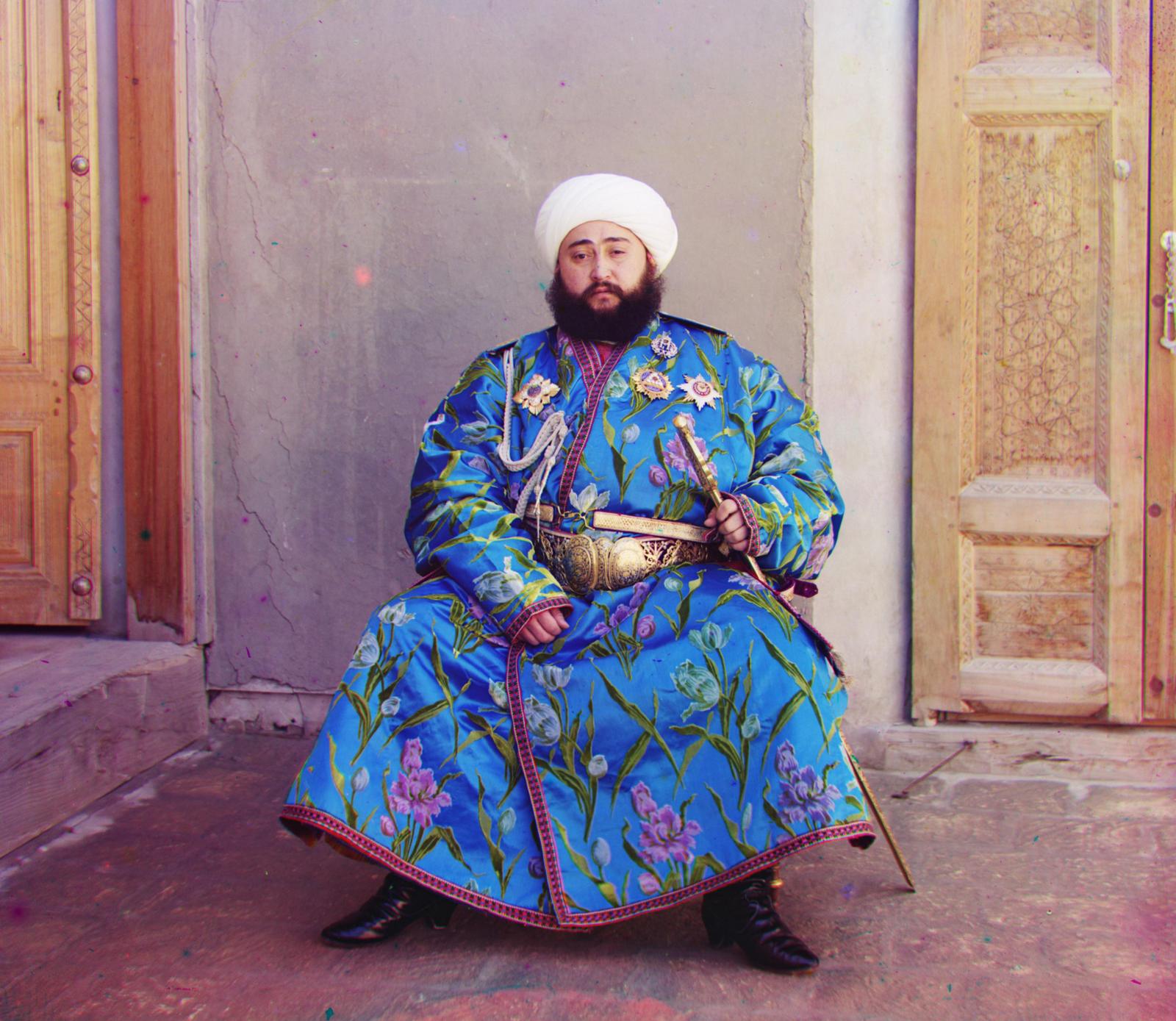
The most important tool for automating contrast is the color channel histograms. Using these histograms, I tried three different constrasting methods: histogram equalization, adaptive equalization, and contrast stretching. Histogram equalization and adaptive equalization produced very cool images but neither produced realistic images (these images were very cool so I included some in the appendix). On the other hand, contrast stretching produced great images when tuned correctly.
Contrast Stretching works by normalizing the a specified range of values rather than the entire range of values. Unlike, histogram equalization, this method is nonlinear and is able to generate a less harsh enhancement of the image. Pictured below are the images with varying limits to the normalizing range:
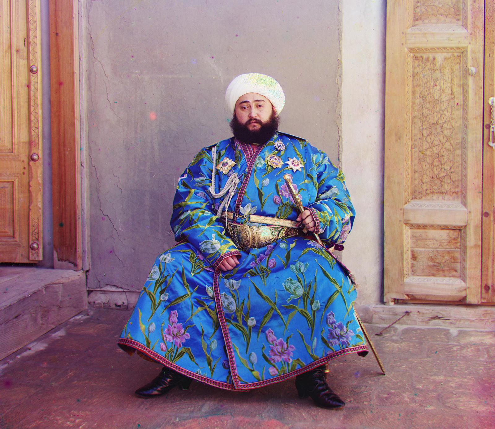

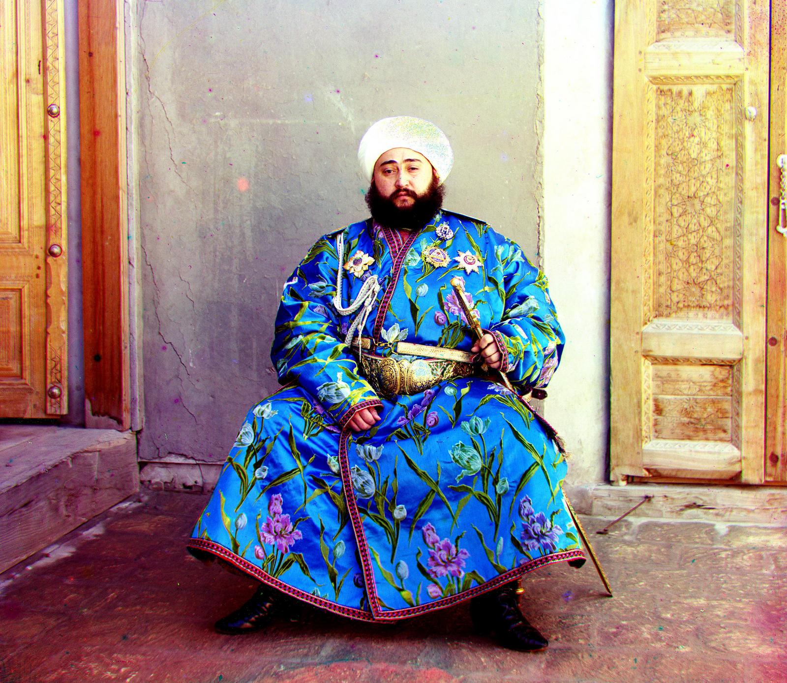
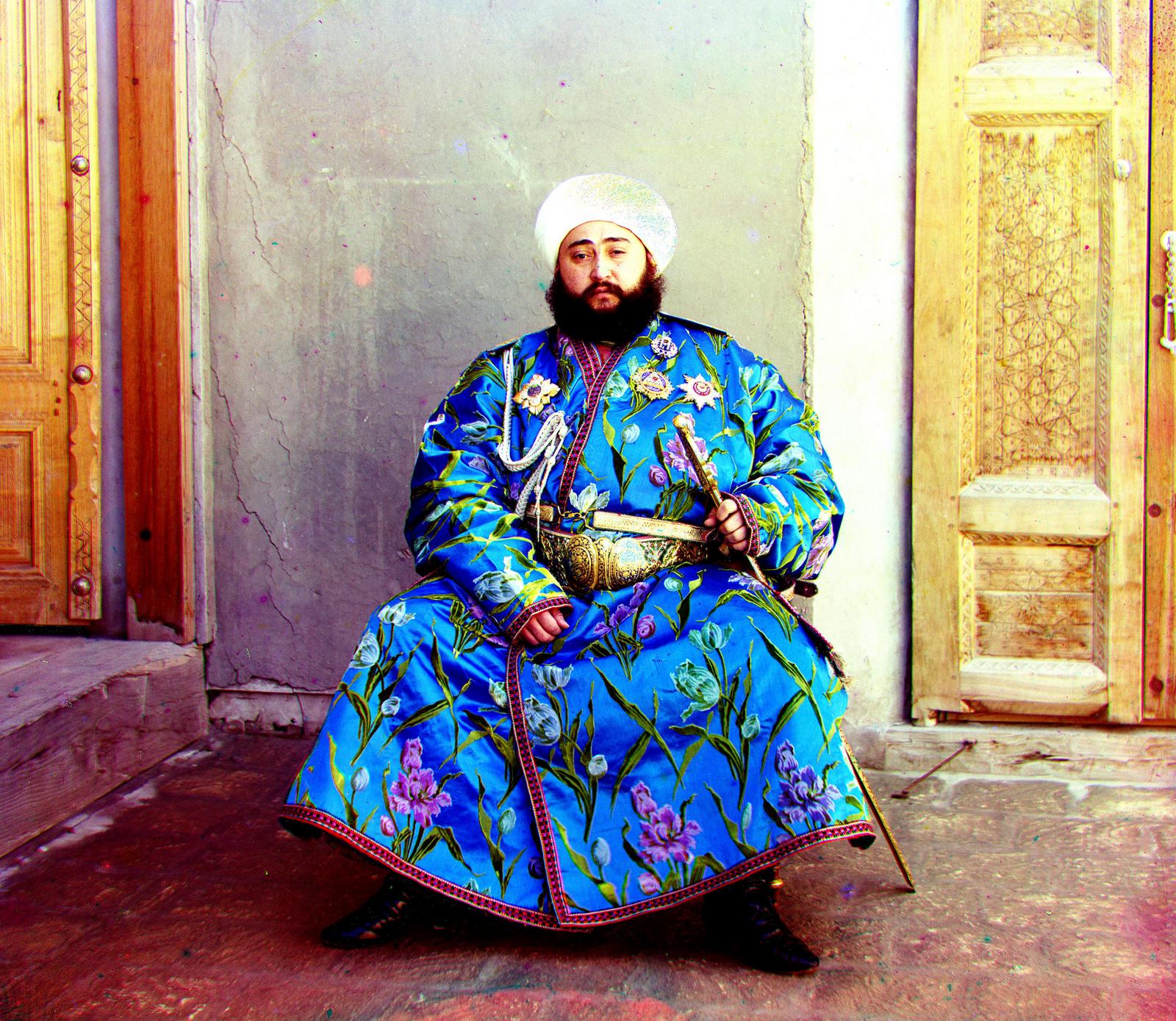
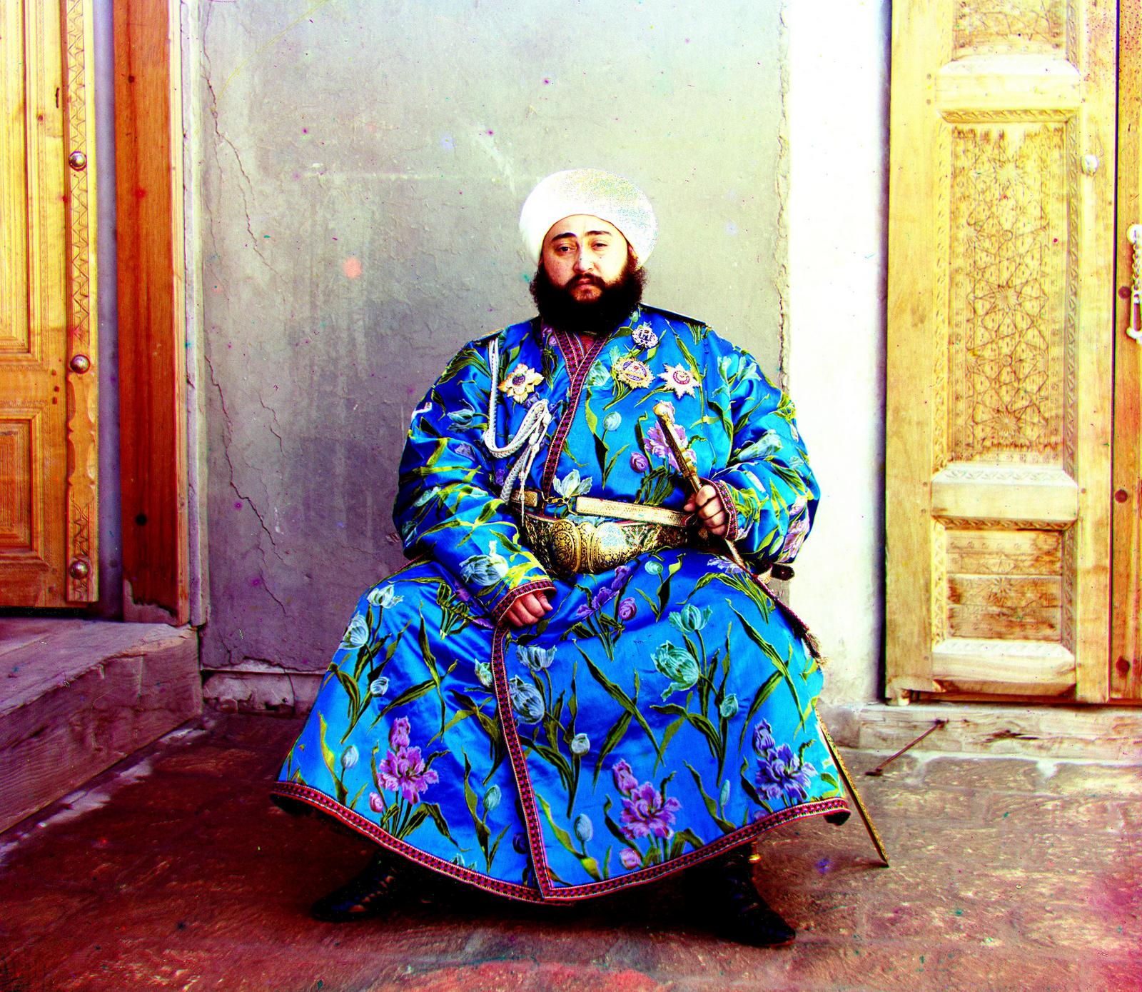
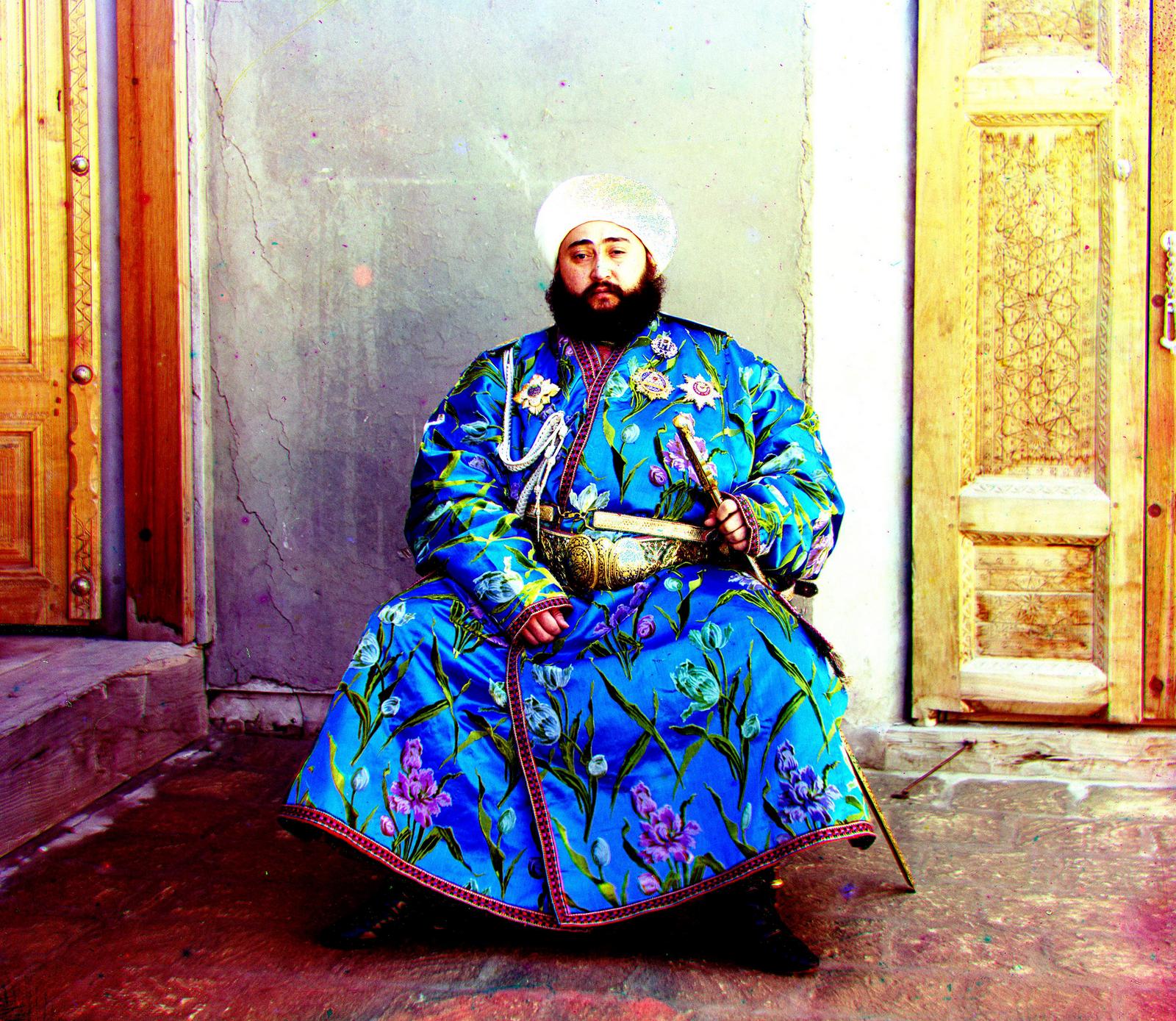

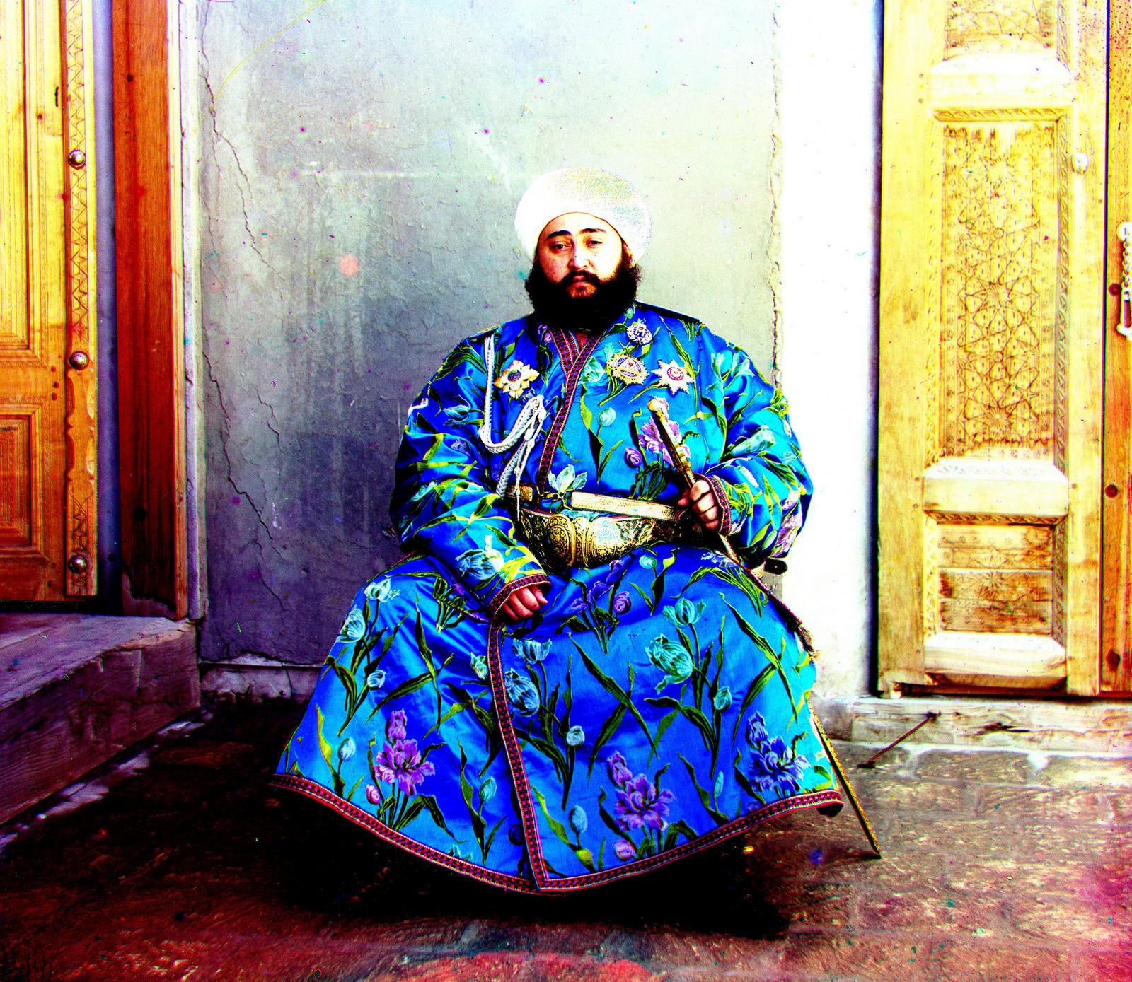
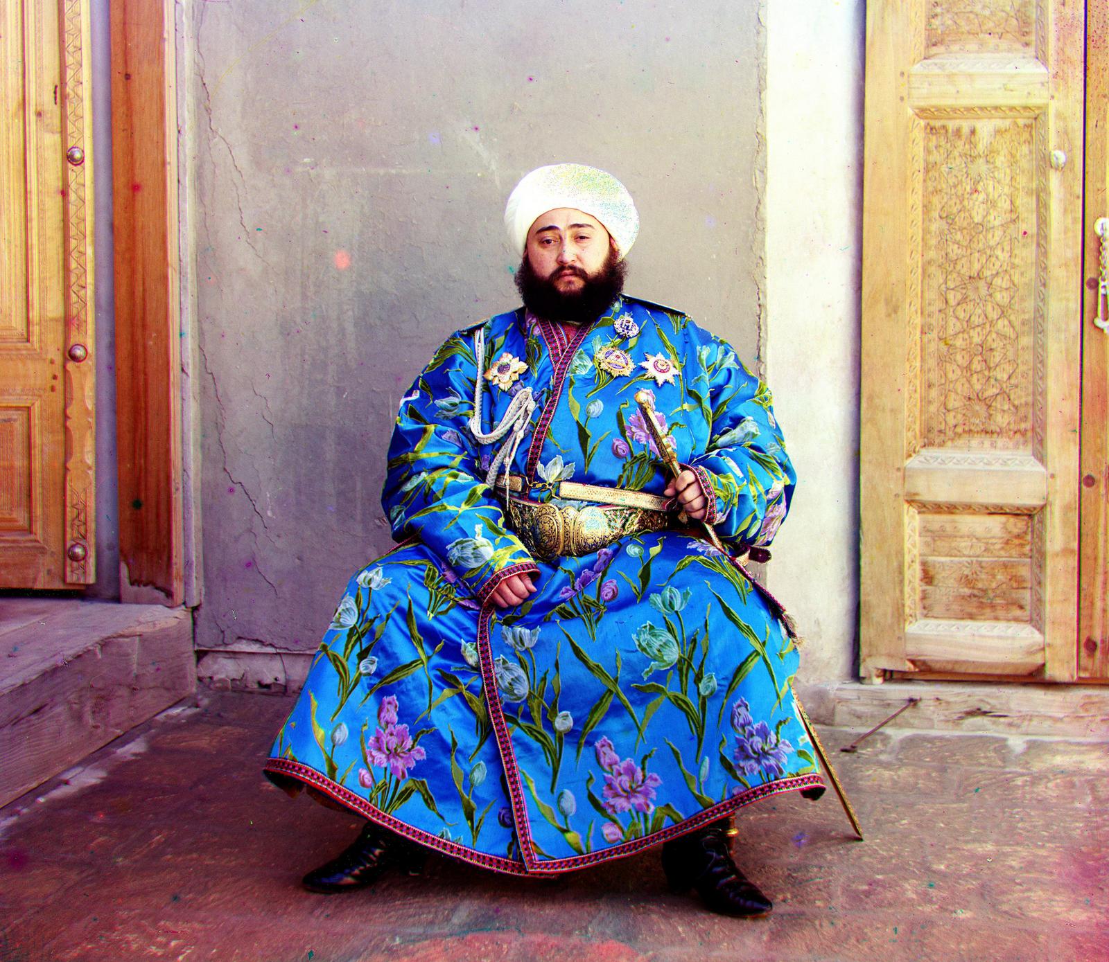
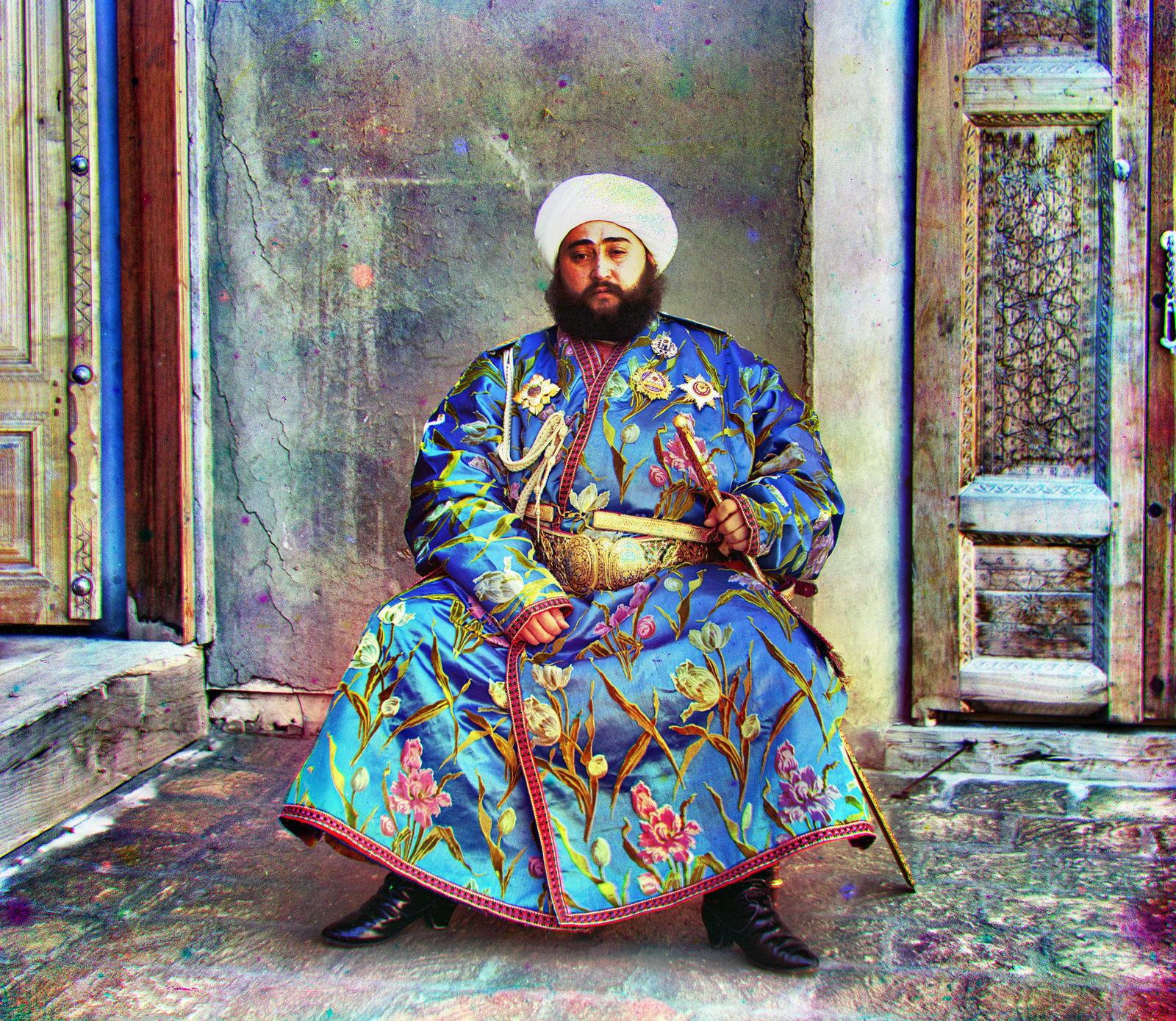
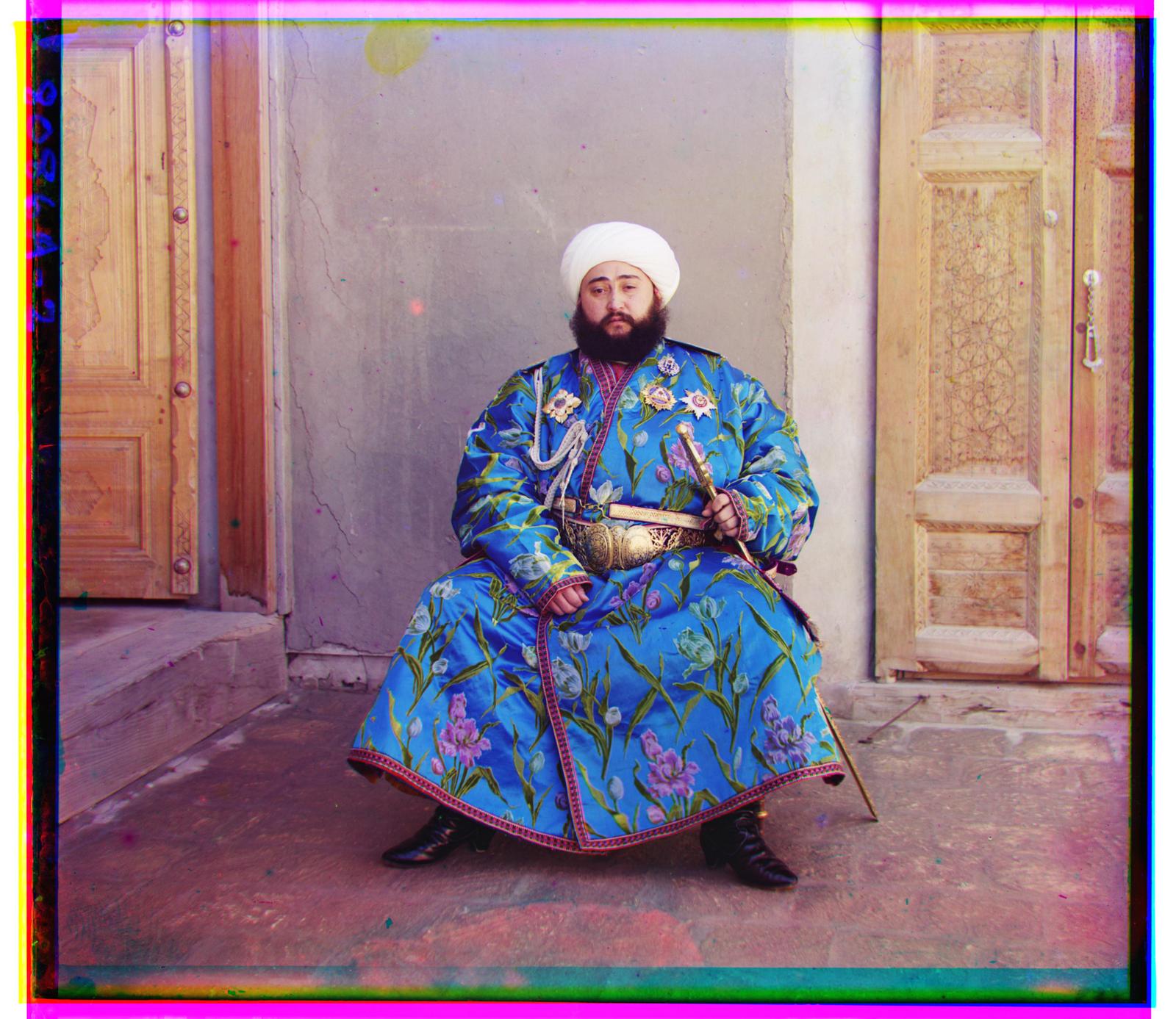
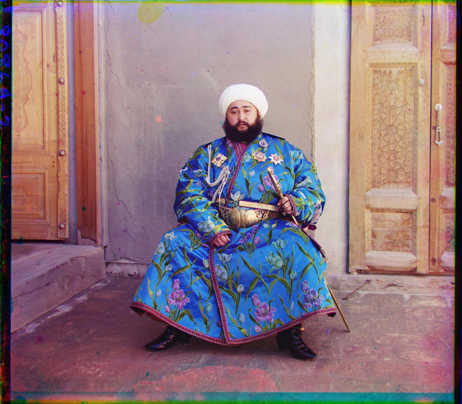
The next feature that I would build would be a saturation controller. I think it would be interesting to experiment with different color mappings or specific hue intensities. Building a saturation and hue adjustment function, then I could manually change these photos to have more realistic or artistic styles. For example, in the photo of Emir, I would like to grayscale everything except for his blue robe.
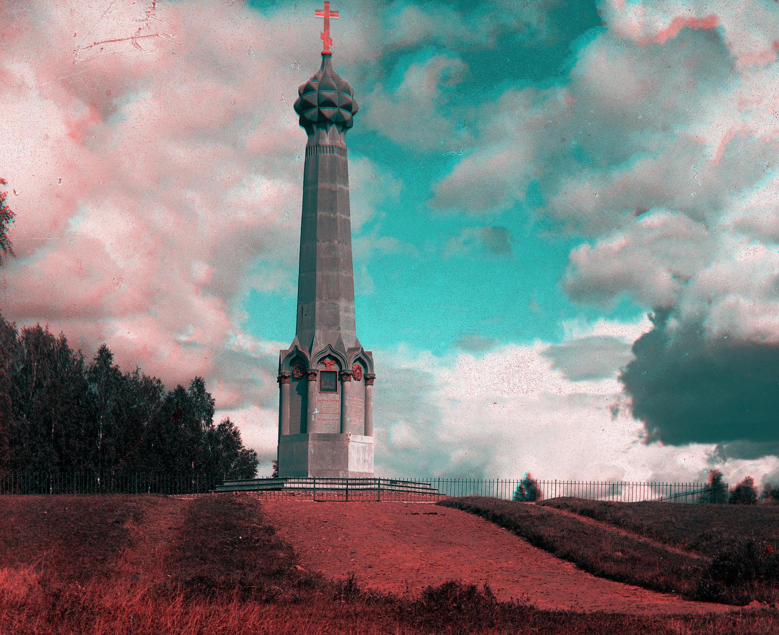
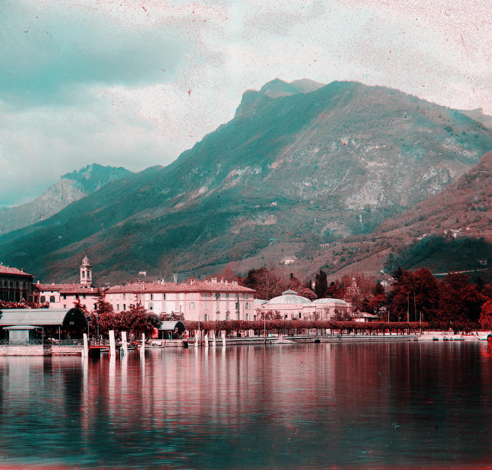
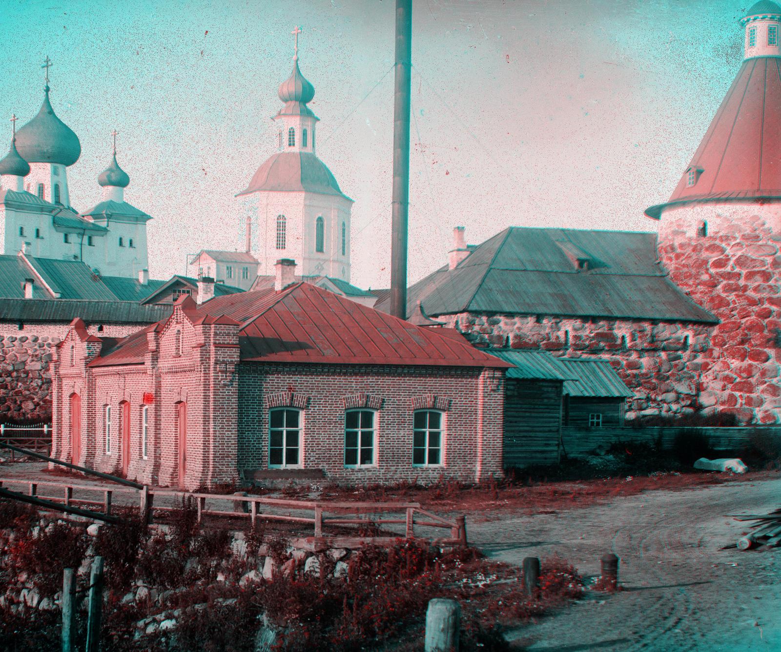
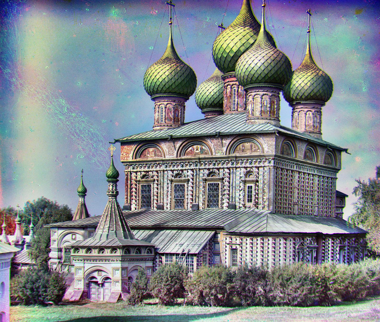
All our pipelining is done, let's see what we got! I highly suggest scrolling to the bottom as well.