Fun with Filters and Frequencies
CS194-26: Project 2
Norman Karr | nkarr11@berkeley.edu
Table of Contents
Fun with Filters
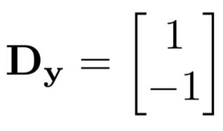
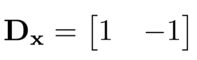
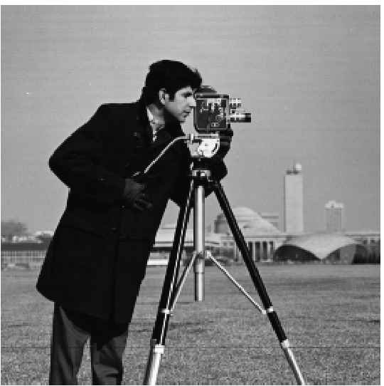
1. Finite Difference Operators
2. Derivative of Gaussian

Sharpening
1. Unsharp Mask Filter
2. Why it's Pseudo Sharpening
Hybrid Images
1. Methodology
2. Fourier Transforms
3. Gallery
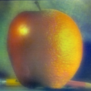
Image Blending
1. Methodology
2. Enhancing and Correcting Color
3. Varying the Mask
4. Gallery
2. Derivative of Gaussians
Above, we solved the noise issue using thresholding. However, there is a better way to minimize noise: low-pass filtering. We first filter out the high frequencies by applying a Gaussian kernel then applying the derivative kernels. Luckily, since convolution is associative, we just just convolve the derivative filter with the gaussian filter and use these new filters are our low-pass edge detectors.
Filters

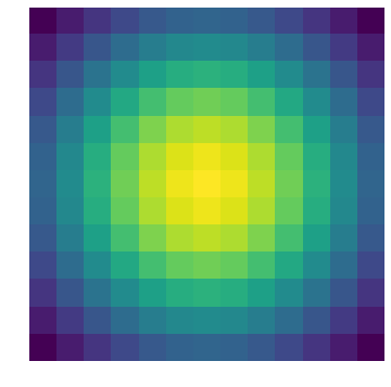
Gaussian Kernel

Gaussian convolved with Dx (DxoG)

Gaussian convolved with Dy (DyoG)
Results
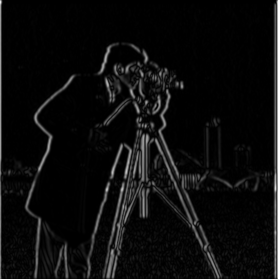
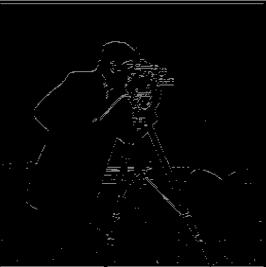
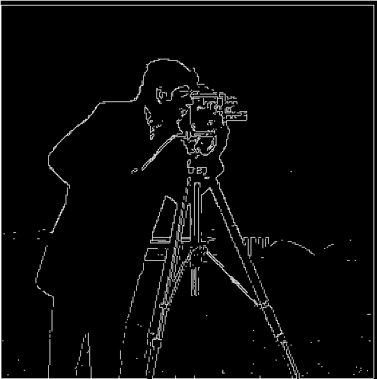
DxoG convolved with Cameraman
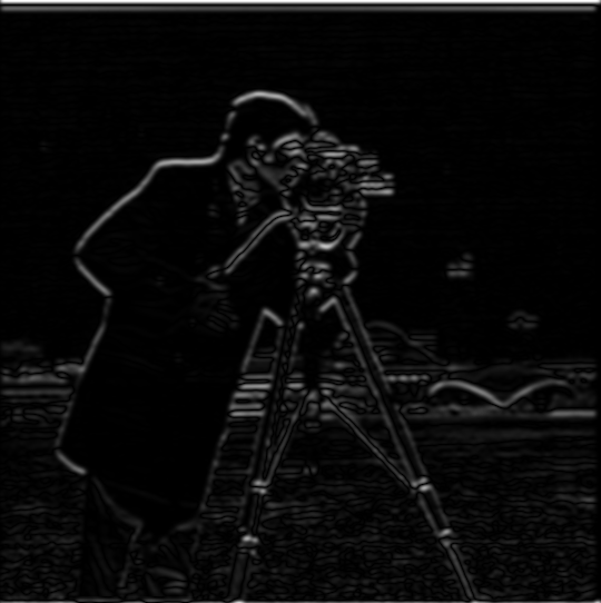
DyoG convolved with Cameraman
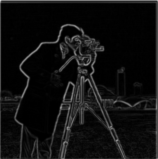
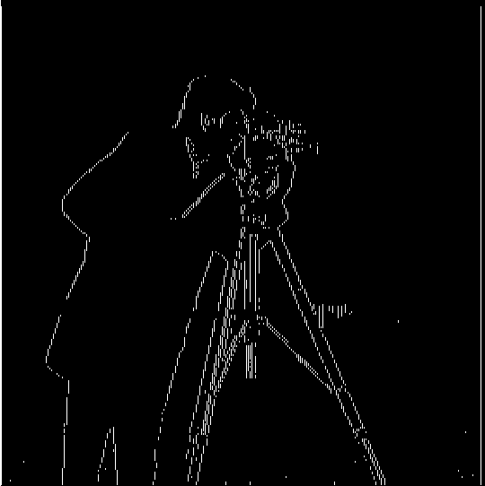
DxoG + DyoG convolved with Cameraman
What differences are there between convolving with finite difference operators versus convolving with derivatives of Gaussians?
The activations without the Gaussian filters have a lot more noise and the activations appear very sharply. The derivative of the gaussian minimizes noise, captures edges more accurately, and produces softer edges. This makes sense because both noise is reduced and edges that are more than 2 pixels across and be detects.
Sharpening
1. Unsharp Mask Filter
One way of "pseudo" sharpening an image is amplifying the high frequency range of an image. To do this, we need a highpass filter to capture the high frequencies of an image. Fortunately, this can be done very easily by applying a Gaussian lowpass filter to the image and subtracting this from our original image. We will have subtracted out low frequencies leaving us with the high frequencies. We then add these high frequencies back into our original image to get a "pseudo" sharpened image.
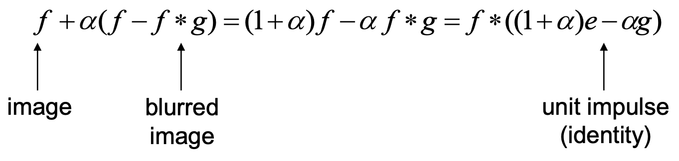
The equation above is the derivation of the unsharp mask filter. The left handside represents adding a scaled highpass filtered image to the original image. The right handside is the actual unsharp mask filter.
Notation: f = image, g = Gaussian kernel, * = convolve
Results
Alpha = 2
Alpha = 5
Alpha = 10
Alpha = 0 (No Sharpening)
Alpha = 0.5

Alpha = 1
2. Why it's "Pseudo" Sharpening
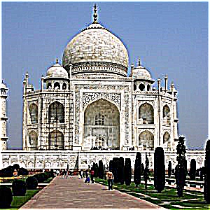
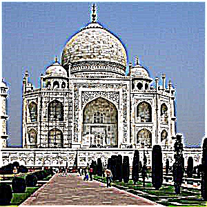
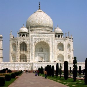
Shown below is an experiment done to show why this filter is pseudo sharpening. We first take our image and blur it. Then from this blurred image we apply our unsharp mask filter in attempt to sharpen the blurred image back to the original. We can clearly see that final result is not able to recreat the original image and thus our sharpening filter is really a pseudo sharpener.
Blurred Image
Sharpened Blurred Image
Original Image
Hybrid Images
1. Methodology
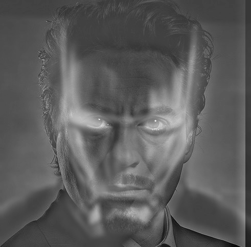
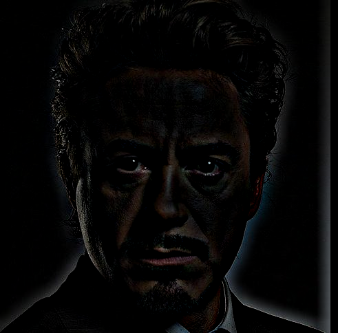
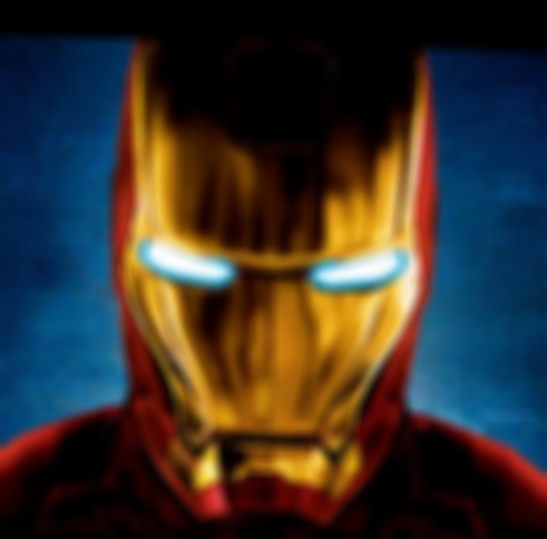
The theory behind creating hybrid images is largely psychological. From close-up, our brain is really good at perceiving high frequencies of a image but from afar, our brain is much better at perceiving low frequencies of the same image. Incidentally, our idea for creating a hybrid image is to lowpass one image and highpass a different image. As long as we can adequately align these two images, combining these two filtered images should be able to make an image that looks like the highpassed image up close and the lowpassed image from afar. From experiments, I found that averaging the two images together normally works better than adding the two images together.
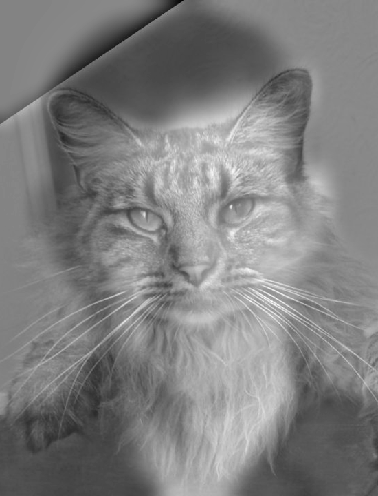
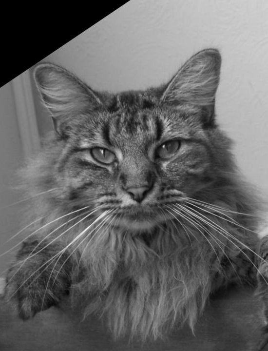
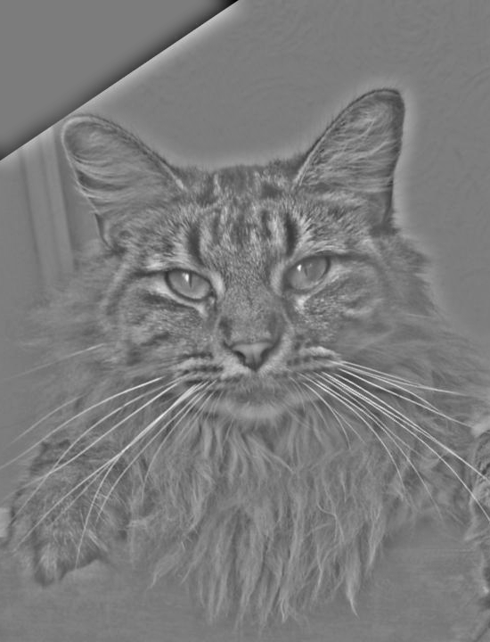
Lowpass Filter
Highpass Filter
Average
Together
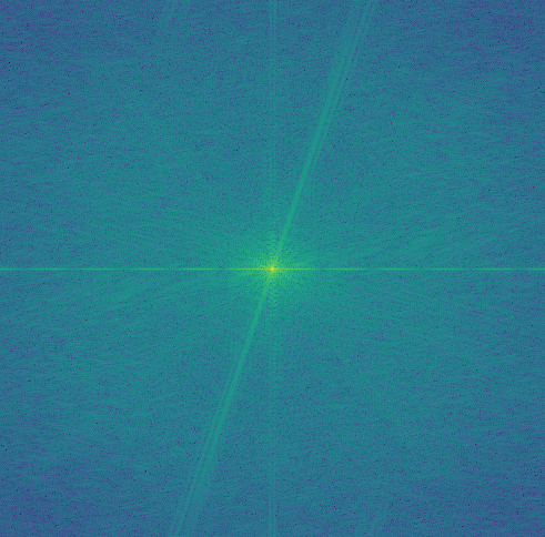
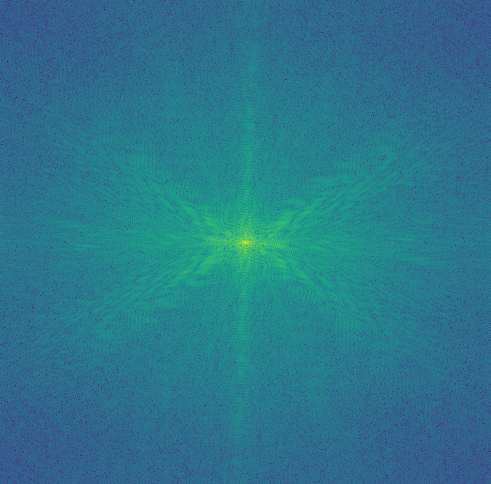
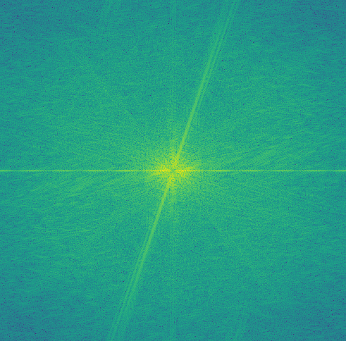
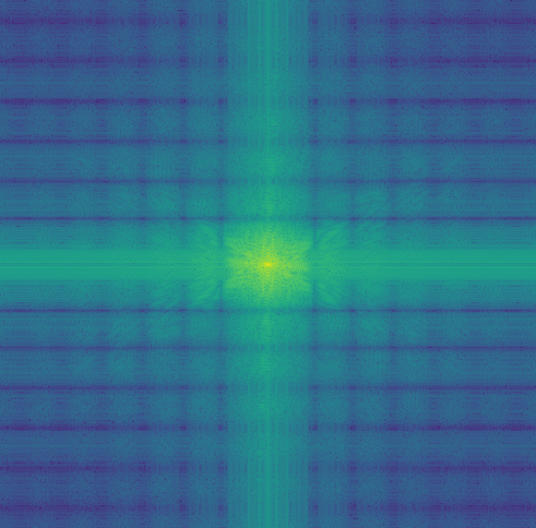
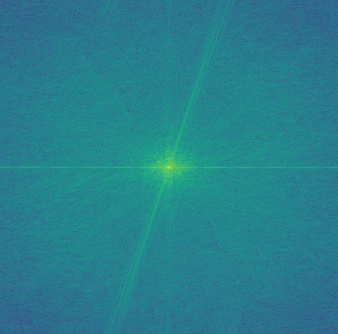
2. Fourier Transform
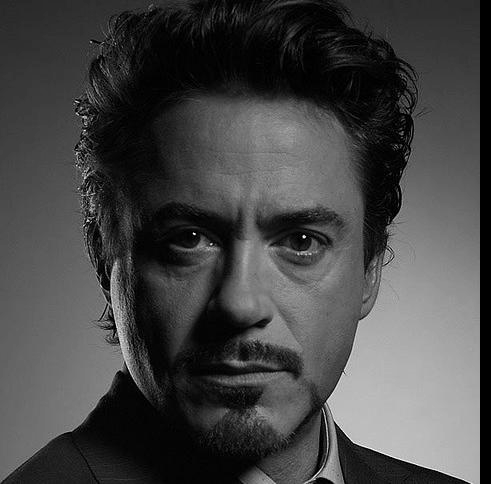
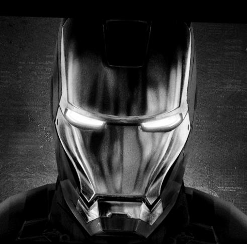
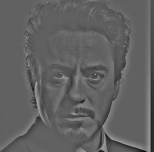
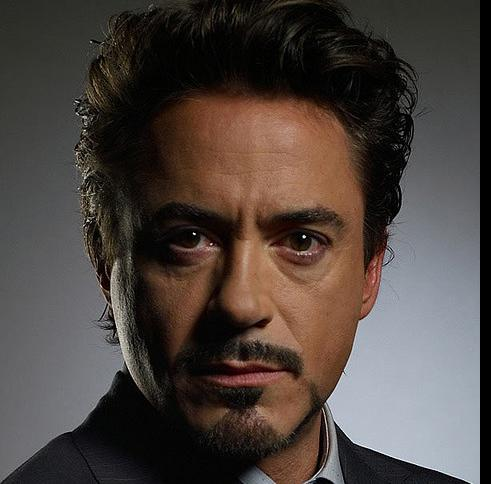
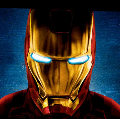
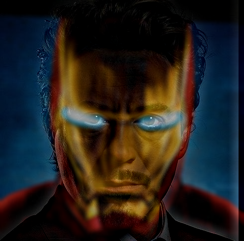
The frequencies present in each image can be visualized with a Fourier transform. Pictured below are the series of images creating a hybrid of Tony Stark and Iron Man. The first row are the processed images and the second row are the corresponding Fourier transforms.
Introducing Color
I made a few attempts at making colorized hybrids and made a few observations. Firstly, very little color makes it through the highpass image thus color is more important for the low Frequency component. Secondly, colors of the two images being combined should be relatively similar otherwise both images break down. In the case of Iron Man and Tony Stark, the colors actually still work because the yellow helmet is still able to complement Tony Starks skin. Lastly, one of the tricks I found to make color brighter was to clip the colorways of the image then normalize across the entire image.
3. Gallery
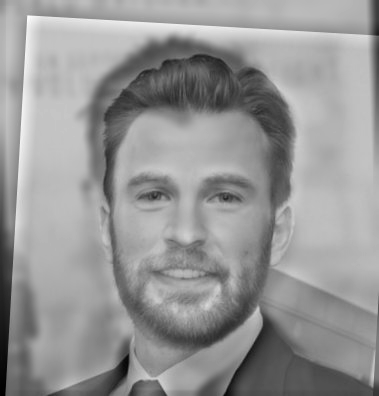
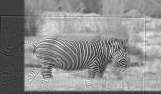
Although I was able to produce a few good results. The better ones being Derek/Nutmeg and Tony Stark/Iron Man and the lesser ones being Hippo/Zebra and Chris Evans/Chris Hemsworth. The Chris's hybrid is okay, from close up it looks like Chris Evans and far away it looks like a different person, it just does not look entirely like Chris Hemswoth. The hippo and zebra was the most severe failure likely because the zebra stripes are apparent enough that you have to go considerably far away to not see the stripes.
Professor Nutmeg
Derek + Nutmeg
Chris Evansworth
Chris Evans + Chris Hemsworth
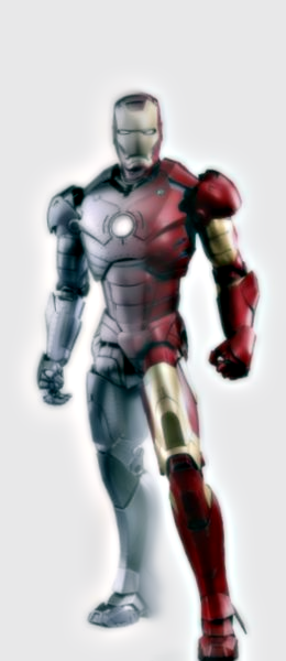
I am Iron Man
Tony Stark + Iron Man Helmet
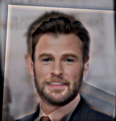
Chris Evansworth (Colored)
Chris Evans + Chris Hemsworth
I am Iron Man (Colored)
Tony Stark + Iron Man
Image Blending
1. Methodology
Our goal is to blend together two images smoothly without creating an evident seam between the two images. One may think that maybe we could just blur the seam but this is not enough because we would lose edges and disrupt both our images. Thus, to properly blend together two images, we will employ a strategy that utilizes Gaussian and Laplacian stacks.
We will start with two images and a mask. Then we will generate a Laplacian stack of image 1, a Laplacian stack of image 2, and a Gaussian stack of the mask. These stacks will be LA, LB and GR respectively. I opted to use a 4 layer stack with sigma (standard deviation) for the Gaussian blur filter as an input. I also maintain a ratio such that the sigma applied to the mask was two times the sigma applied to the images. At each layer, we multiply element-wise the mask with the first image and (1-mask) with the second image then we add the two resultant images together to get a new stack, LS. The results of each layer are shown below:
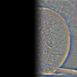
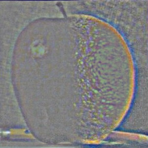
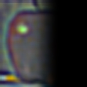
Results of Laplacian Stacks
(a)
(b)
(c)
Column (a) are the results the Laplacian stack LA multiplied by the mask's Gaussian stack.
Column (b) are the results of the Laplacian stack LB multiplied by 1 minus the masks's Gaussian Stack.
Column (c) is the row-wise sum of column (a) and column (b).
**Note that the final row is just to demonstrate raw slicing, these images are not used in final calculations**
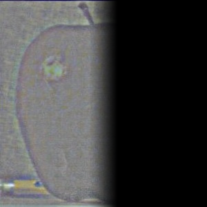
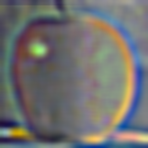
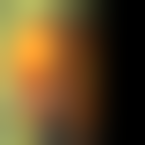
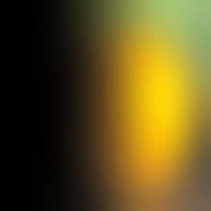
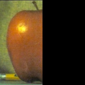
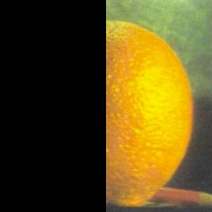
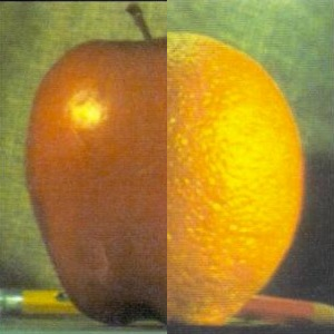
The Oraple
Our final blended image can then be made by summing across each image in the LS Stack. The final image is then normalized such that pixel values are between 0 and 1.
Shown on the right is the blending of an apple with an orange with a left window mask
2. Enhancing and Correcting Color
One of the first problems I noticed when I tried combining other images was that if the background colors did not match, it is still clear that there are two images. I fixed this issue by writing a piece of code that would offset the color of the first image such that its background matched the background color of the second image. This produced much more uniform results but would have awkward exposures. As a result, I applied a contrast stretch to the image to finalize the color correction.
Basic Blending
Matching Background
Adding Contrast Stretching
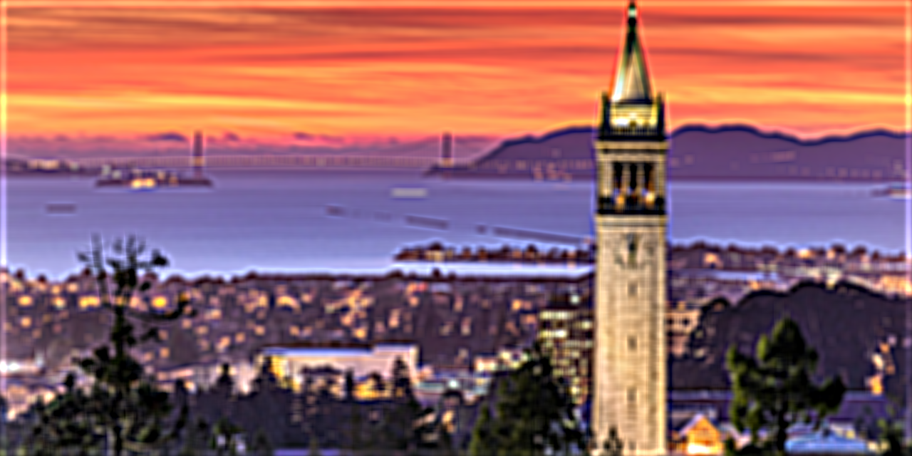
**Gray-to-Color Gradient Idea**
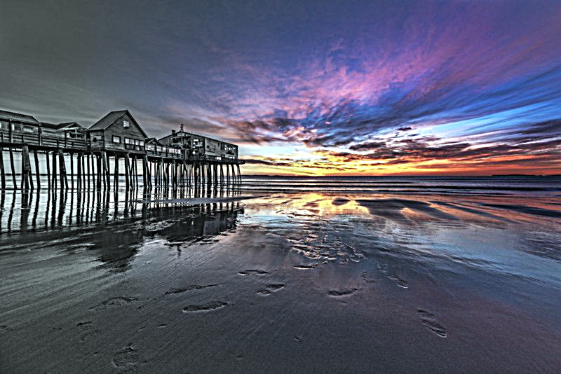
The images above are the result of two different Iron Man images: an image of the silver Mark 2 armour blended with the red and gold Mark 3 armour. However, this idea of fading from gray to colored gave me an idea of taking on image and creating a color gradient on it. This can easily be done with the blending algorithm by taking an image and a grayscaled version of that image, and then running the blend algorithm on the two images. This then creates a gradual grayscale-to-color blend across the masks. An example is seen below in the gallery with a beach photograph.
3. Varying the Mask
One of the nice things about the masks is that it is really easy to create different masks and then blending will automatically blend all edges of the mask. Thus, we can create and apply many different mask shapes to achieve different structures of blending.

Window Mask
Circle Mask
Snake Mask
4. Gallery
The Oraple
Apple + Orange + Window Mask
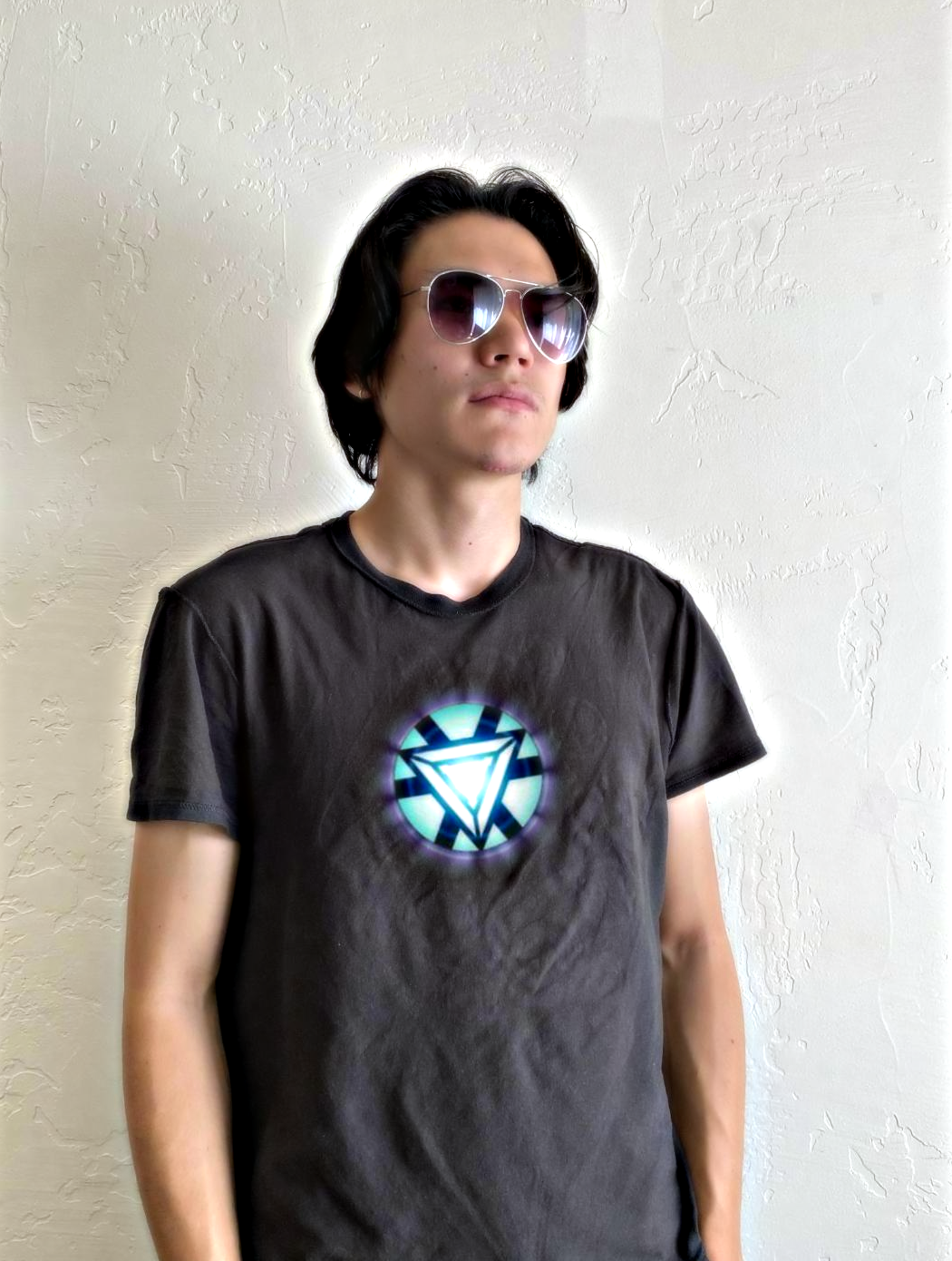
A New Avenger
Norman + Arc Reactor + Circle Mask
In the Shop
Mark 2 + Mark 3 + Window Mask
Colliding Galaxies
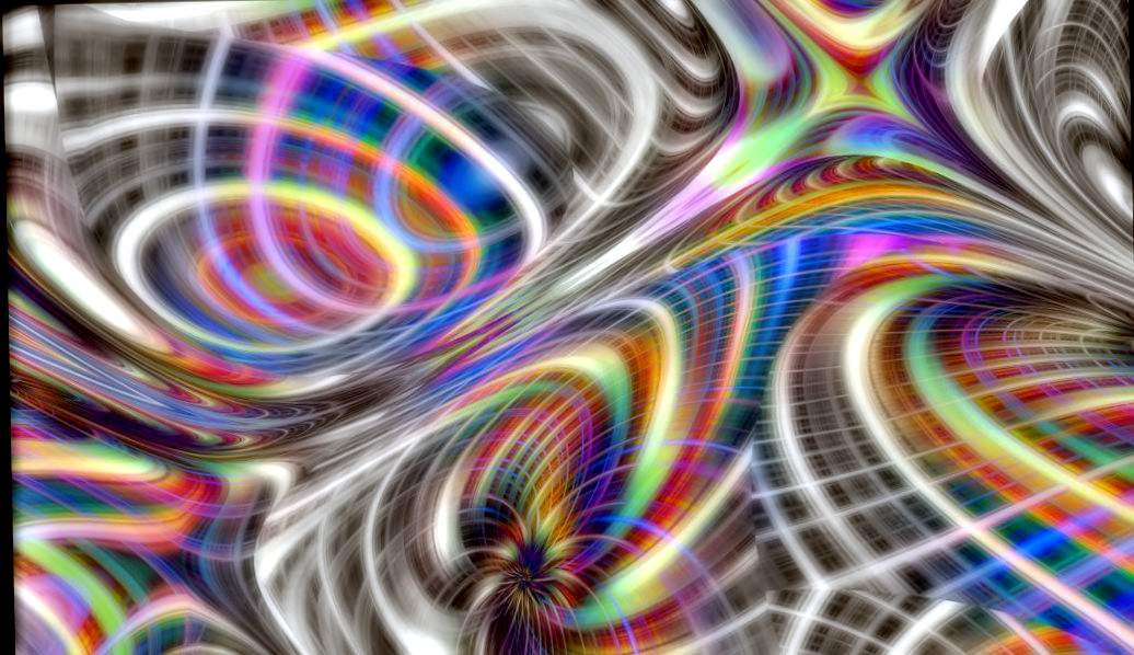
Colored Pattern + Different Grayed Pattern + Snake Mask
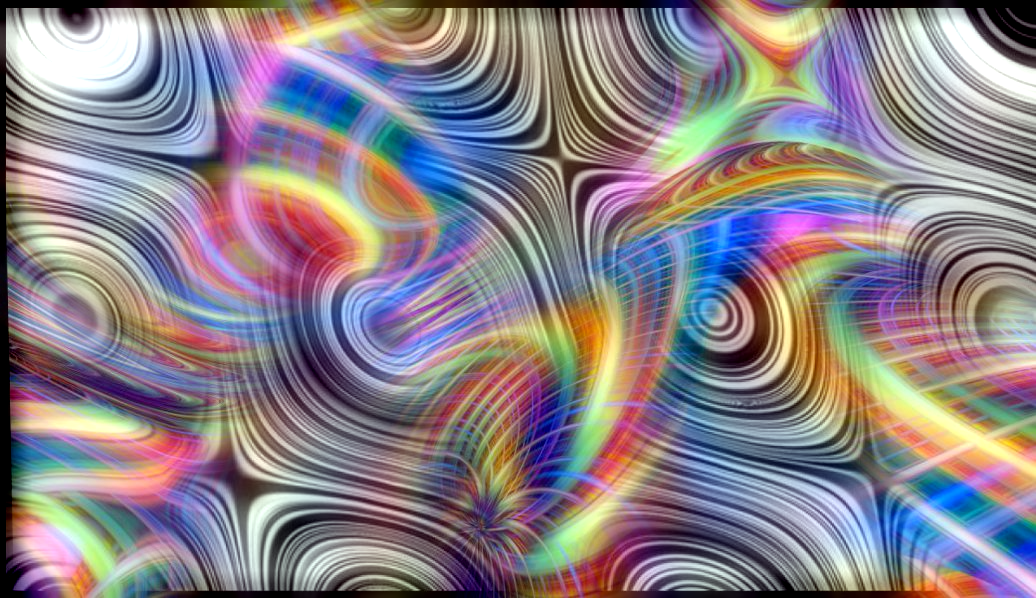
Kaleidoscope Prism
Colored Pattern + Same Pattern Grayscaled + Snake Mask
Journey to the Sea
Beach + Gray Beach + Soft Window
What did I learn and think was cool/interesting?
My favorite part about this project was the blending portion. This method of blending images allows for a lot of artistic creativity on how I combine images. I have flexibility in which images I use as well as what kind of masks I can use. The idea is simple but the results are fantastic.
The most useful thing I learned I think was the gaussian filters. Applying the gaussian filter is incredibly useful for many different things such as feature extraction and anti-aliasing when downsampling.