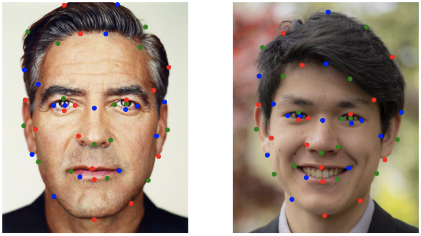
For the two images I define a distinct set of key points that has a corresponding point in each photo. For example, the bottom red key point represents the bottom of the chin for both faces.
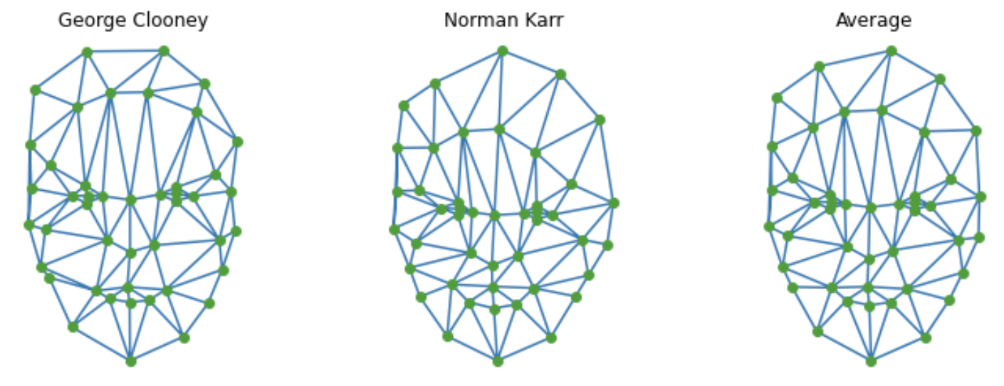
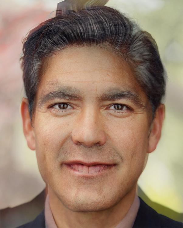
Pictured above is the triangulations of the keypoints from George Clooney, Norman Karr, and the average shape of the two faces.
**Note: the actual meshes used for morphs also includes key points for the 4 corners of the image to capture the backgrounds**
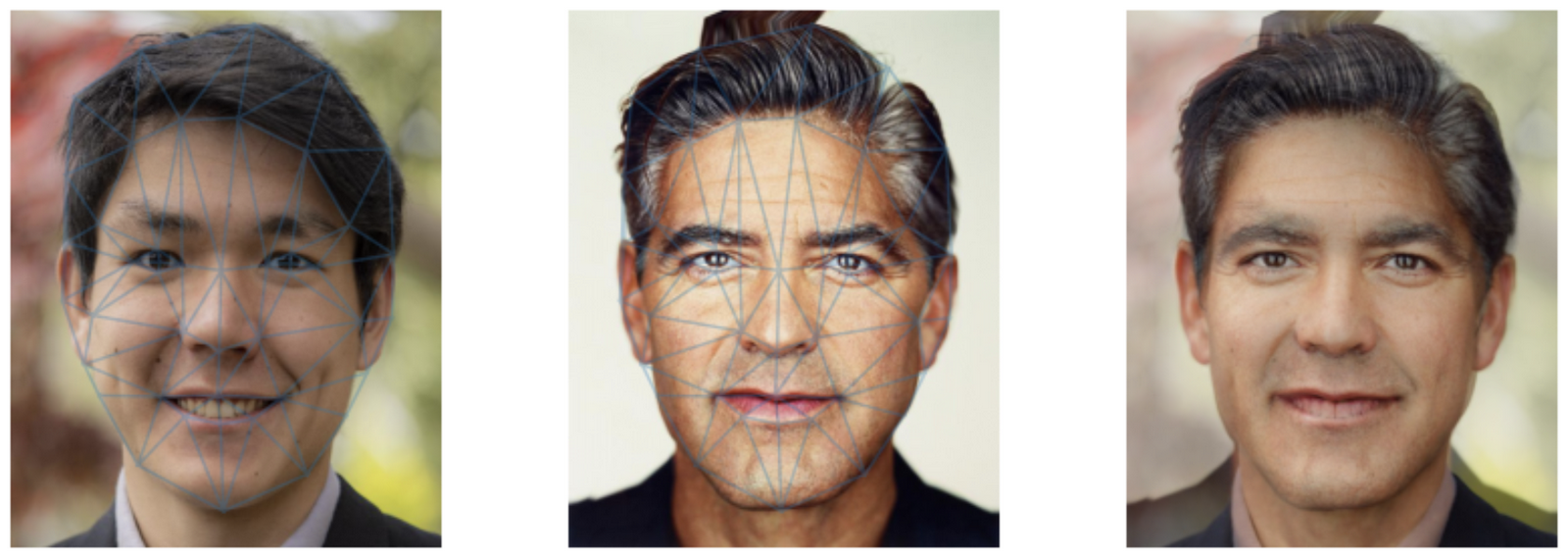
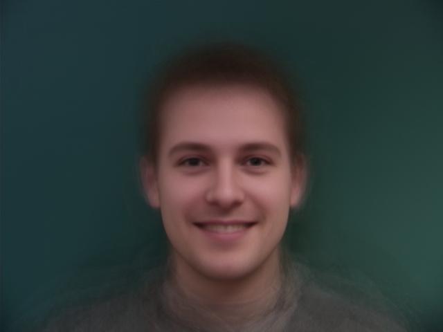
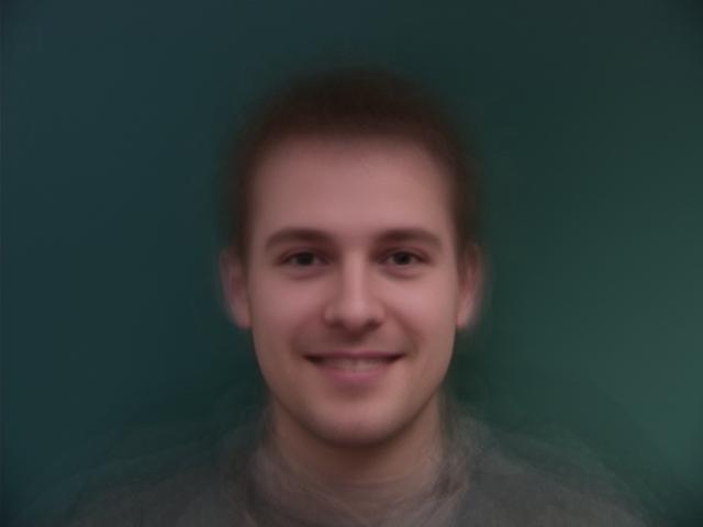
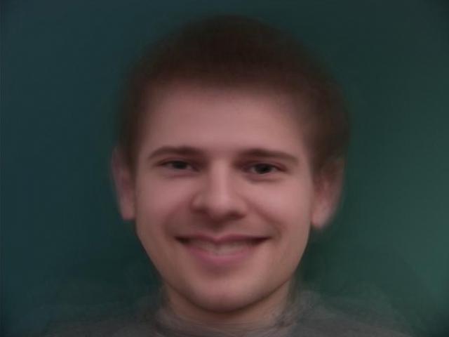
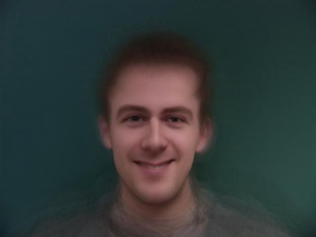
Norman morphed into the average shape
Clooney morphed into the average shape
Cross dissolve of the two averaged faces (The Midway Face)
Observations:
The morph sequence is pretty good but there are some obvious shortcomings. The first is that the teeth of my smile seem to ghost in. Secondly, there is no space between George Clooney's hair and the image boundary so as this part morphs, the background inherits just black pixels. Thus, there is an obvious remnant of Clooney's hair getting ghosted away in the background.
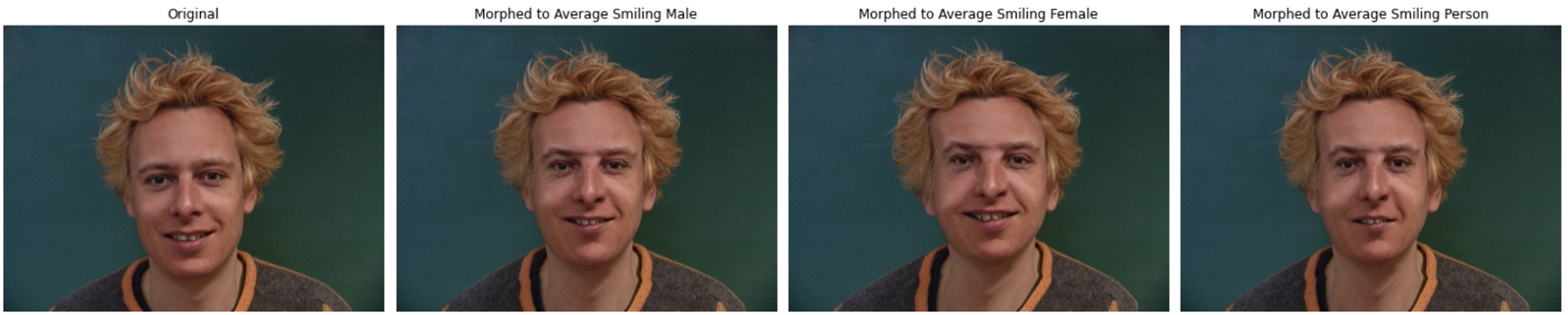
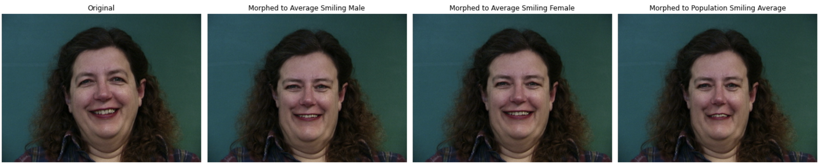
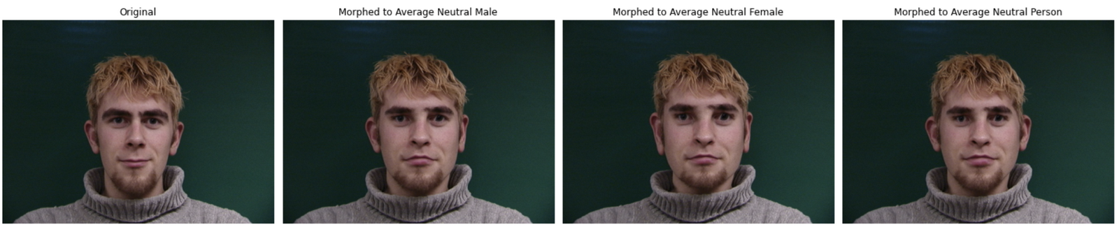
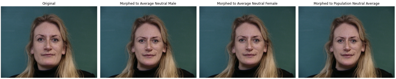
**Note that the total average faces look dominantly male likely because this database contains 33 males and 7 females**
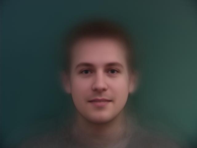
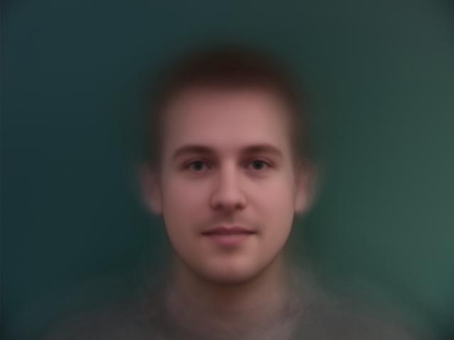
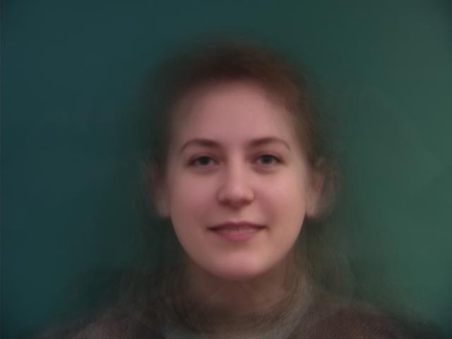
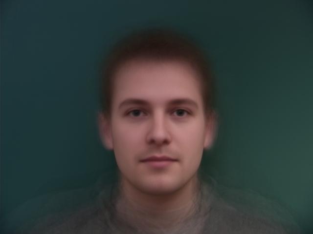
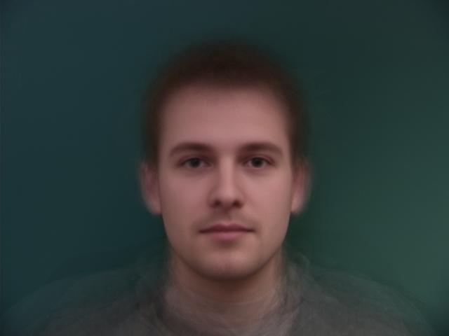
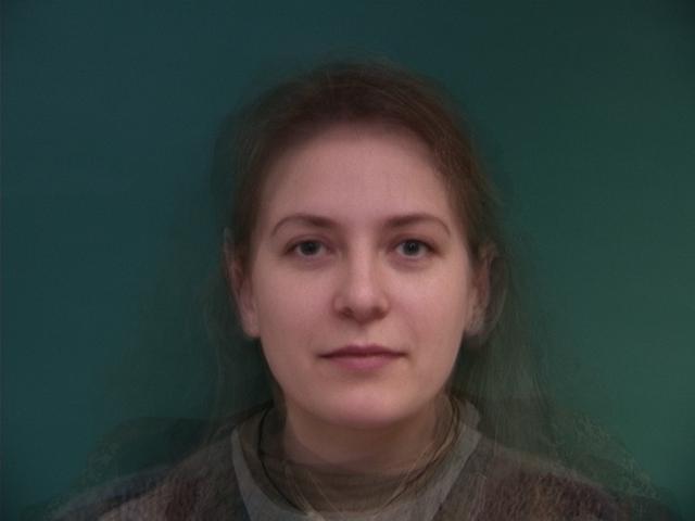
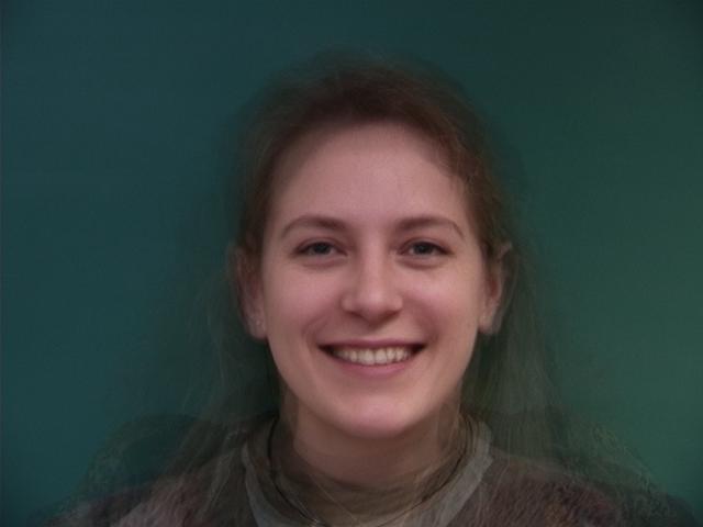
Although some of these morphs definitely leaning towards creepy, there are some good things happening. For example, most faces being morphed to the average faces become more uniformly round and symmetrical. The same can be said for my face as well except for my dimples make the distortion look a little bit too apparent.
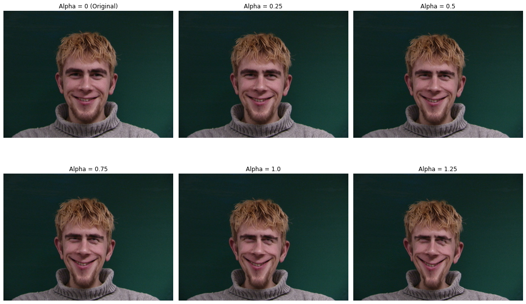
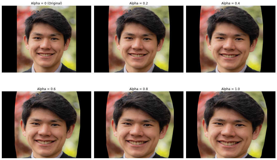
Once we have an average shape, we can also create caricatures of individuals. Caricatures are basically representations of people where their distinct features become more pronounced; i.e. enlarging Obama's ears. We can perform a similar operation with our key point representations of faces. We subtract the mean face from our face to get a vector representing how our face deviates from our mean. We then add a scaled version of vector back into our face to make our unique features more pronounced.
**Note: I defined my own new set of key points because the key points defined from the Danes' dataset was not sufficient to account for hair properly.**
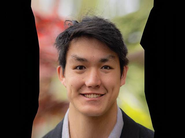
This was a simple addition for bells and whistles. I put together a morph of the BAIR Computer Vision faculty by following the same process as before but for multiple faces. Extensions to this would be to include the entire BAIR faculty but that would involve manually selecting many keypoints. I'll take suggestions for a background song/sound to add to the video.
With a simple process of keypoints and images, I thought it would be interesting to apply it to objects other than faces. I decided to apply it to objects with a hilt. I selected keypoints corresponding to hilts and blades so that the morphs would sync up based on the different pieces of the objects.
The danes dataset did not have enough faces to produce an interesting set of principle components from PCA. So to experiment with PCA, I used "The Extended Yale Face Database B" which is a dataset with 16128 images of 28 different faces under various different lightings and poses. I filtered out images that have super dark lighting and very low contrast but otherwise kept all images for PCA.
Pictured below are the first 16 eigenvectors of the dataset
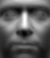
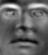
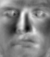
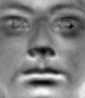
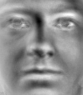
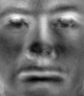
The idea of PCA is that you calculate a specific set of vectors that capture the most information about the dataset. Thus, we should be able to compress, and then reconstruct, each face into the eigenvector basis produced from PCA.
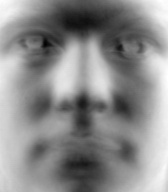
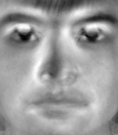
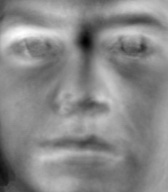
Original Image
(Image was present in dataset)
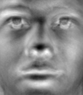
Compressed representation
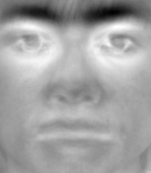
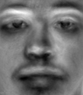
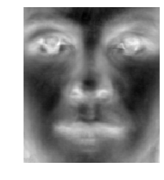
Reconstructed image from compressed vector
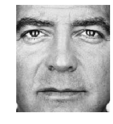
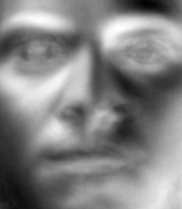
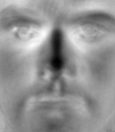
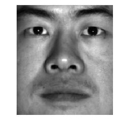
Original Image
(Image not present in dataset)
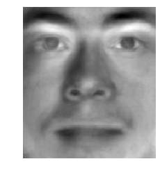
Compressed representation
Reconstructed image from compressed vector
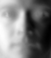
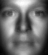
The results shown below are the results from using the 16 previously calculated eigenvectors. The first pair of images are for an image that was present in the dataset used for PCA. The second pair of images is an attempt to compress an out of distribution image of George Clooney. The reconstruction of the in-distribution image is not perfect, the 16 eigenvectors was enough to recapture the original expression and general face structure of the image. Unfortunately, the reconstruction of George clooney is pretty underwhelming. I suspect it may be because the image is out of distribution, the image may not be aligned as well with the data, or 16 eigenvectors was simply not enough eigenvectors to represent George Clooney.